
AI Outlook: Adoption, Capital Cycles and the Price of Expectations
JQTrading Research | October 6, 2026 | Strategic horizon: 3-5 years | Cycle horizon: 6-18 months
AI is becoming an economically important service, but the industry’s ability to build capacity has to be matched by customers’ ability and willingness to pay. Our outlook is constructive on durable adoption and cautious about assuming that all layers of the supply chain can sustain exceptional returns. Technology success and security returns can diverge for years.
This expanded report follows the sequence: revenue, capital spending, historical analogies, supply chains, model economics, chip competition, memory cycles, warning signals, valuation, employment, scenarios and allocation. It brings the complete 24-exhibit historical and industry set together with six additional financial and analytical exhibits.
Our base case is growing adoption with unequal value capture. The upside case requires reliable production use, measurable customer returns and healthy utilization. The downside case combines weaker paid demand with rigid financial commitments. Historical analogies inform these scenarios but do not date the market peak.
Evidence is labeled at the exhibit level. Dated company disclosures, retained reference estimates, image-derived historical illustrations and hypothetical calculations serve different purposes. The report preserves every reference exhibit while explaining disagreements and unsupported assumptions rather than silently turning them into verified facts.
| JQTrading view | What would change the view |
|---|---|
| Long-term adoption: constructive | Persistent failure to deliver measurable paid outcomes |
| Near-term industry earnings: selective | Broad improvement in utilization and cash conversion |
| Valuation: requires discipline | Prices reset or durable earnings catch up |
| Peak timing: no calendar forecast | Converging evidence across demand, pricing and orders |
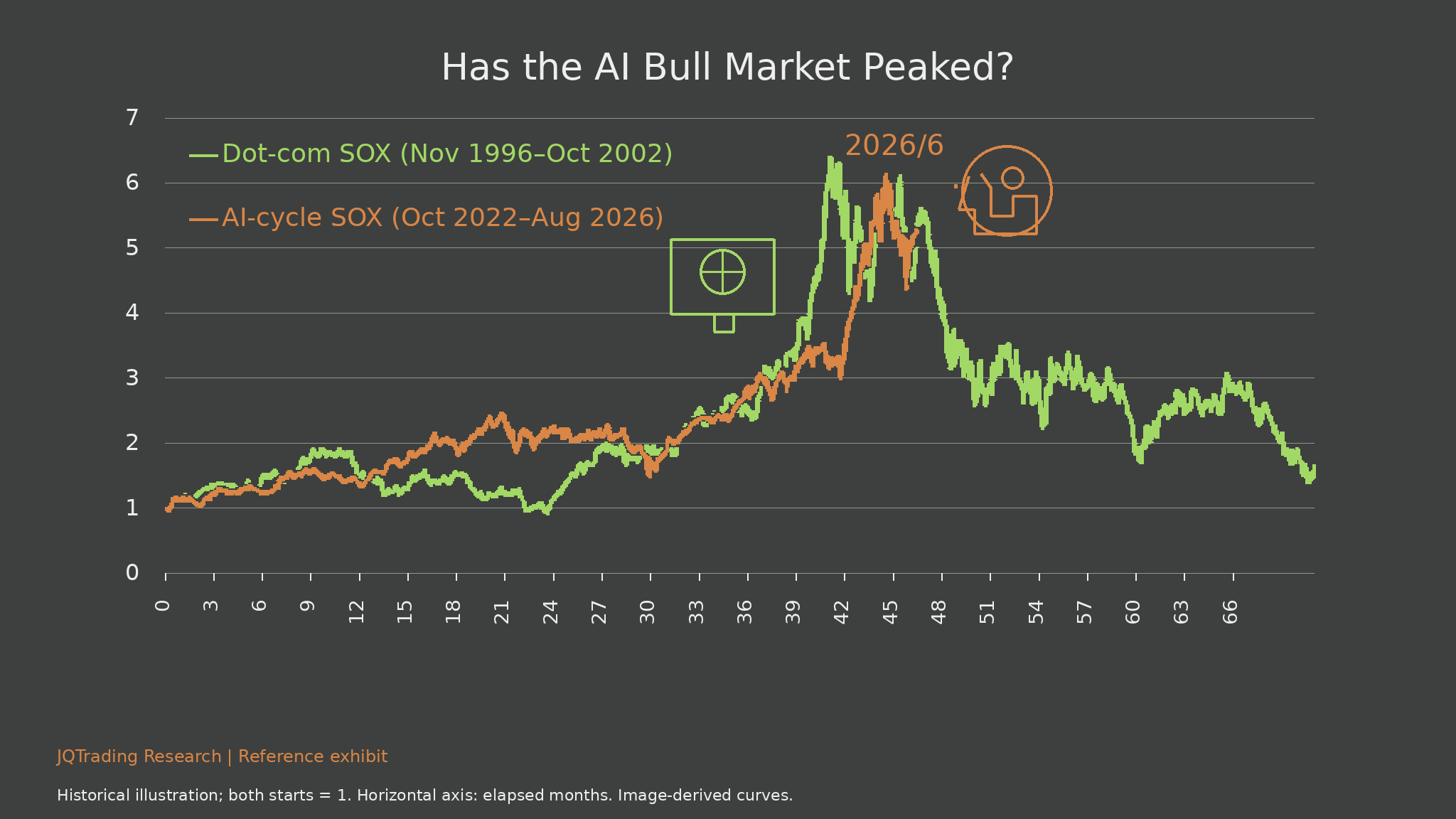
Exhibit 01. Has the AI Bull Market Peaked?
What the exhibit shows
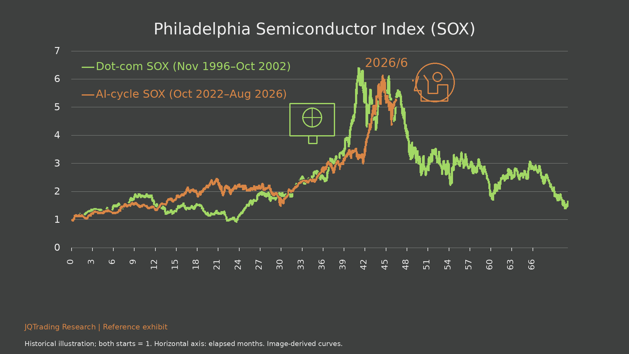
The opening SOX comparison aligns the November 1996-October 2002 internet cycle with the October 2022-August 2026 AI cycle. Each begins at one. Both reconstructed peaks are around six times the starting level, equivalent to a gain near 500%, rather than a 600% gain.
Investment interpretation
The resemblance raises the right question: how much durable earnings growth is required to support the cumulative revaluation? It does not establish that the current cycle must follow the historical decline. This opening exhibit is repeated with fuller baseline analysis in Section 3 so that no part of the reference chart set is omitted.
Limits and monitoring
The horizontal axis is elapsed months. The two series belong to different calendar periods. Their outlines were reconstructed from images; exact daily returns and peak dates cannot be derived reliably from these curves.
1. Revenue growth supports the opportunity, not every valuation
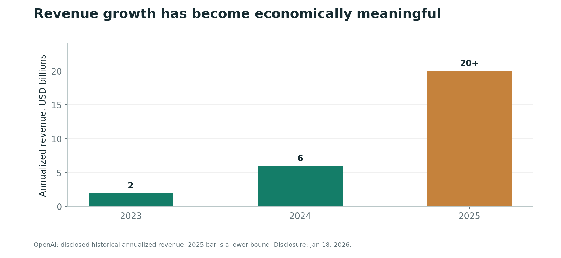
OpenAI disclosed annualized revenue of approximately $2 billion in 2023, $6 billion in 2024 and more than $20 billion in 2025. Anthropic disclosed that its revenue run rate crossed $47 billion in May 2026. These dated observations demonstrate significant commercialization; they are not estimates of either company’s current October revenue.
Annualization extrapolates a recent revenue pace. It is not recognized full-year revenue, contracted backlog or free cash flow. Nor should figures from different dates be used as a synchronized market-share comparison. Rapid growth can coexist with large training, inference and customer-acquisition costs.
For investors, the next questions are renewal rates, incremental revenue per customer, gross profit after serving costs, cash collection and dependence on a few large partners. A high headline growth rate supported by discounting or temporary credits is less valuable than recurring growth supported by customer productivity.
The complete model-revenue tables that follow put the opportunity in context. Their main contribution is to show the speed of commercialization; their principal risk is confusing annualized sales pace with sustainable recurring cash generation. Uneven sampling dates and inconsistent definitions limit claims about deceleration or competitive ranking.
Exhibit 02. OpenAI: Historical annualized revenue
What the exhibit shows
The historical annualized-revenue sequence is approximately $2B, $6B and more than $20B for 2023, 2024 and 2025. The last bar marks a lower bound. Annualization describes a recent sales pace and should be separated from audited recognized revenue.
Investment interpretation
Commercialization at this scale supports an enduring demand opportunity. Investors still need customer retention, serving economics and cash conversion to decide how much of that demand becomes distributable earnings.
Limits and monitoring
These are dated historical observations, not an October 2026 estimate. The figure does not measure profit, free cash flow or the full industry market size.
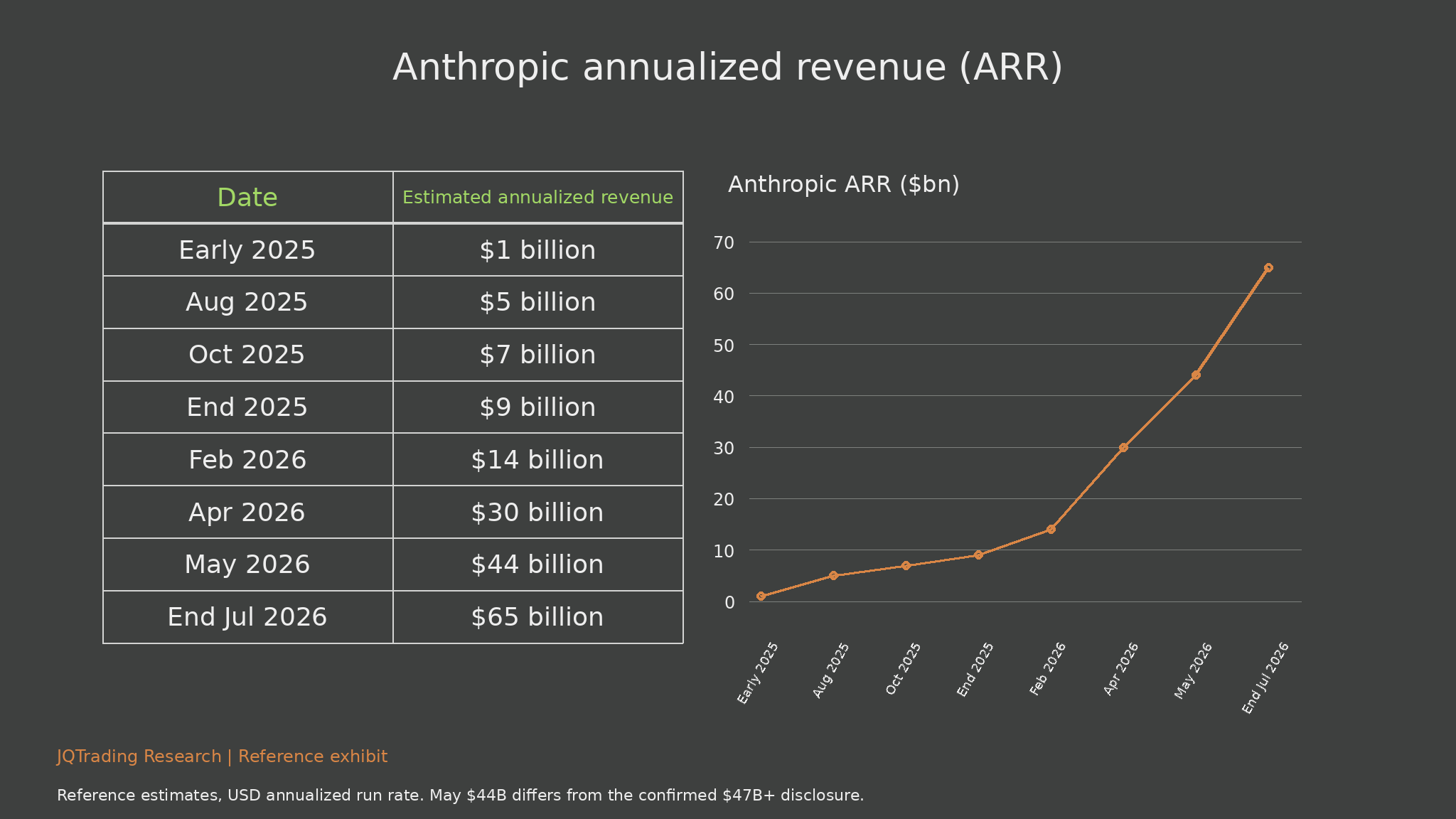
Exhibit 03. Anthropic ARR table and growth curve
What the exhibit shows
The reference sequence runs from $1B in early 2025 to $5B in August, $7B in October and $9B at year-end; it then lists $14B in February 2026, $30B in April, $44B in May and $65B at end-July. All values are annualized estimates, not completed-year sales.
Investment interpretation
The series captures a commercialization acceleration associated with coding and agent workflows. Its sequential changes cannot be read as monthly growth rates because intervals differ. The confirmed May disclosure exceeded $47B; the original $44B cell is retained for completeness and explicitly reconciled here.
Limits and monitoring
Apart from the separately checked May disclosure, the full timeline has not been independently reconstructed from accounting records. Do not infer an exact growth slowdown, market share or audited revenue total from the curve.
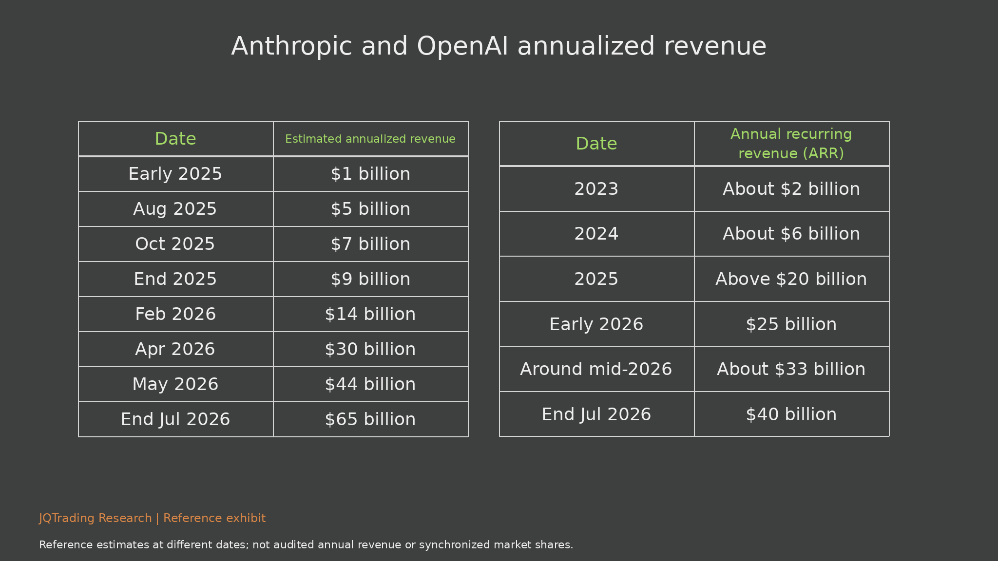
Exhibit 04. Anthropic and OpenAI ARR comparison
What the exhibit shows
The comparison retains the same Anthropic timeline and an OpenAI sequence of about $2B in 2023, $6B in 2024, $20B+ in 2025, $25B in early 2026, $33B around mid-year and $40B at end-July. The columns use different observation schedules.
Investment interpretation
Model providers have moved beyond experimental monetization, but a side-by-side table is not a clean market-share ranking. A model can grow quickly while its contribution margin or financing requirements worsen. Coding and agents may deepen usage; price competition may offset that usage growth.
Limits and monitoring
The reference annualization convention uses four weeks of API revenue multiplied by thirteen plus monthly subscriptions multiplied by twelve. Company definitions may differ. The 2026 OpenAI estimates and July comparisons are retained as reference estimates, not independently confirmed current figures.
2. Capital spending is a commitment to future utilization
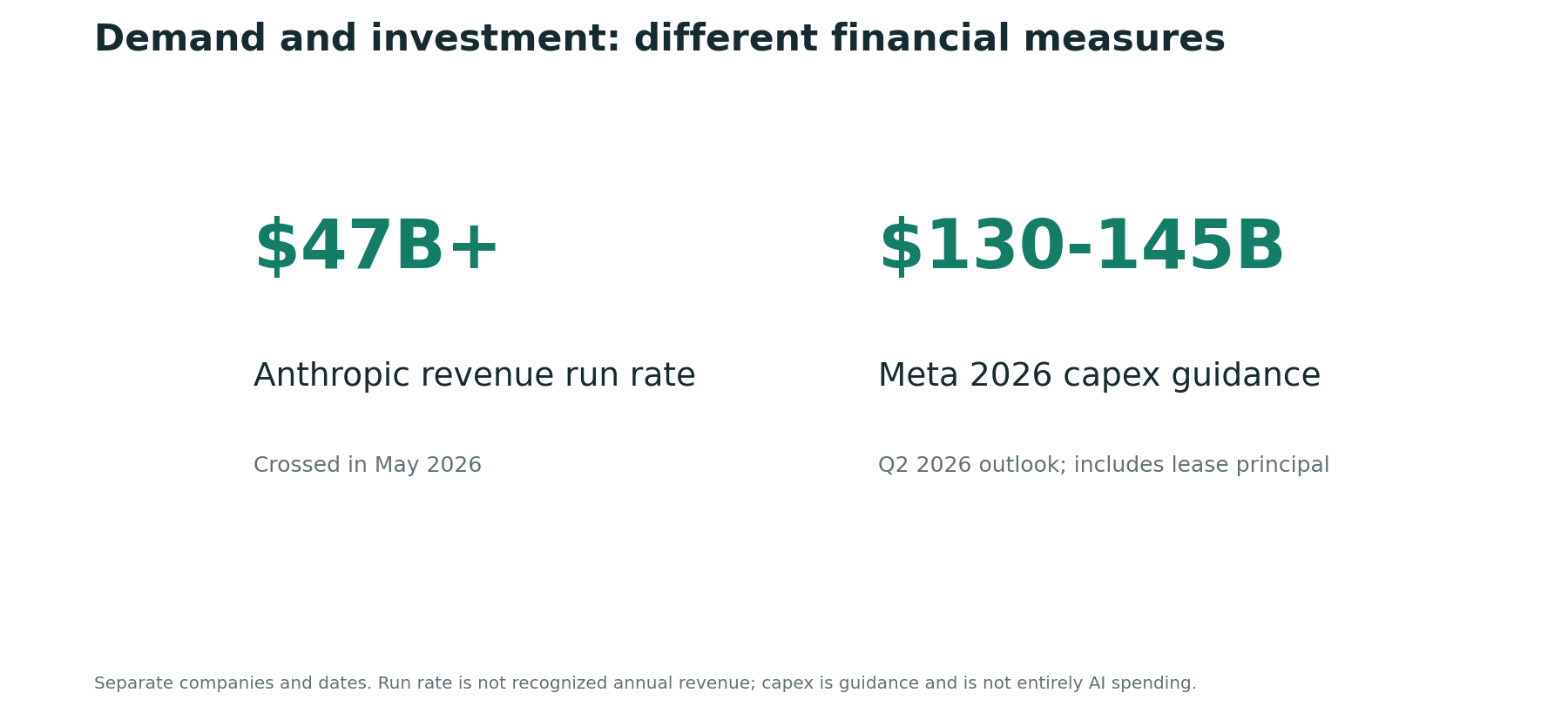
Meta’s Q2 2026 outlook placed full-year capital expenditures, including finance-lease principal, at $130-145 billion. This is company-wide guidance, not a realized AI-only expenditure total. Its importance lies in the scale and persistence of infrastructure commitments.
A mature advertising or cloud business can fund infrastructure from existing cash generation. A standalone model company or specialized compute lessor may depend more heavily on external financing. These different balance sheets should not be grouped into one undifferentiated AI spending story.
There is also a double-counting problem: model revenue, cloud revenue and chip revenue can represent different stages of the same customer dollar. Adding them does not produce a clean measure of final demand. Equity investments, cloud purchase commitments and financing partnerships can strengthen an ecosystem without proving independent end-user profitability.
As capacity enters service, depreciation, interest, power and operating expenses become harder to defer. Cash spending can peak before depreciation fully appears in reported earnings. We therefore monitor returns and utilization across an asset’s life, rather than judging a buildout solely by one quarter’s operating margin.
Large investment programs can survive weak short-term share performance when their sponsors have strong existing businesses. However, return discipline eventually requires a connection between customer spending, asset utilization and after-tax cash generation. The reference aggregate-spending claim is discussed as a hypothesis requiring reconciliation, not treated as an independently established total.
Exhibit 05. Model demand and capital investment: Different measures
What the exhibit shows
The two panels distinguish a May Anthropic revenue run rate above $47B from Meta full-year capital-expenditure guidance of $130-145B issued with Q2 2026 results. Meta guidance includes finance-lease principal.
Investment interpretation
The central mismatch is between cash earned from serving demand and cash committed to building capacity. This juxtaposition illustrates scale; it is not a return-on-investment ratio between the companies. An infrastructure sponsor can also earn AI-related returns through its existing advertising or cloud business.
Limits and monitoring
The figures cover different businesses, dates and financial definitions. Meta expenditure is company-wide and not wholly AI. The broader reference claim that four hyperscalers spend over $700B and consume most operating cash flow requires a consistent company-by-company cash-flow reconciliation before adoption.
3. The dot-com analogy is a stress test, not a clock
The historical index, valuation and company-return comparisons point to a useful pattern: an application boom can become an infrastructure boom, and the real technological opportunity can survive a collapse in the prices paid for it. Capital can migrate upstream as bottlenecks become valuable. Suppliers then inherit sensitivity to the investment budgets of their customers.
Elapsed-time overlays are highly sensitive to the starting month. Indexing two series to one removes their initial scale, but does not align interest rates, profits, valuation, market composition or the stage of adoption. Moving the dot-com baseline changes how much apparent upside remains. That instability prevents us from using the overlay as a market-top forecast.
Historical winners also introduce survivorship and corporate-action problems. Current company names may not represent the same economic entity traded decades earlier. Acquisitions, delistings, spin-offs, splits and dividends can change a comparison materially. A sequence of sector leadership is more credible as a hypothesis than a precise return target derived from selected historical stocks.
The practical signal is a combination: infrastructure leadership broadens, customers struggle to earn returns on their spending, and suppliers begin to lose pricing or order momentum. Rotation alone is insufficient. It can also occur because profitable demand is expanding faster than supply.
We examine initial valuation first, then the 1994 and 1996 SOX baselines, then historical market phases and the complete company-return table. This progression preserves both the optimistic and cautious interpretations. Neither is allowed to become a precise price target by itself.
| Analogy | Appropriate use | Common error |
|---|---|---|
| Normalized index paths | Compare volatility and cycle shape | Treat elapsed time as a forecast |
| Initial P/E levels | Test sensitivity to entry valuation | Ignore rates and earnings definitions |
| Application-to-hardware rotation | Investigate investment incentives | Declare a peak from leadership alone |
| Historical drawdowns | Stress liquidity and position size | Assign the same loss to current firms |
Exhibit 06. S&P 500 index and trailing P/E
What the exhibit shows
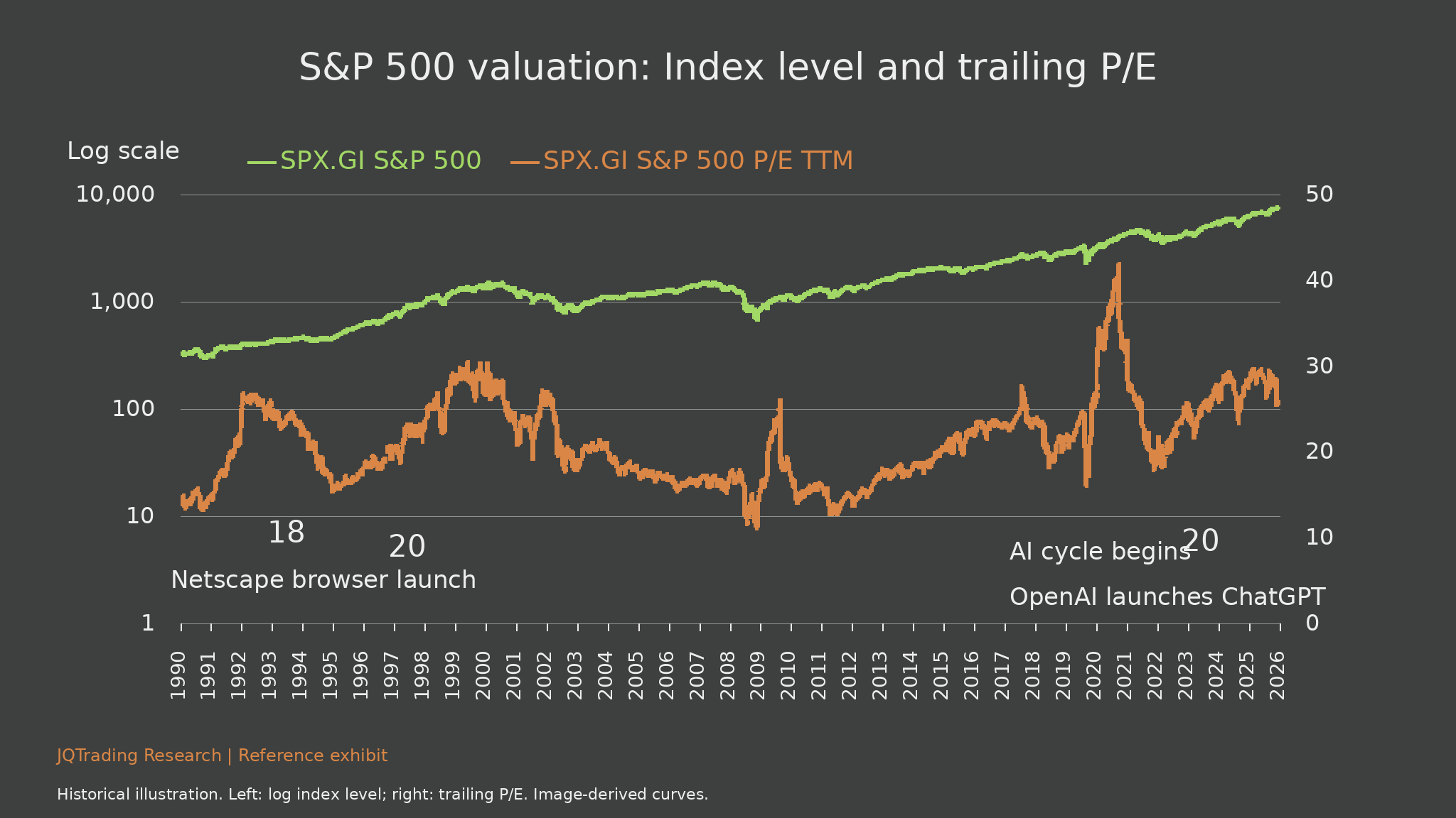
The green line represents the S&P 500 index on a logarithmic left axis. The orange line uses the separate right axis for trailing-twelve-month P/E. Reference annotations put initial multiples near 18 around the 1994 internet starting point and near 20 around late 1996 and the 2022 AI starting point.
Investment interpretation
Different initial valuations change how a subsequent rally should be interpreted. Moving the historical baseline toward a similar multiple can make an analogy less mechanically optimistic. However, equal S&P multiples do not establish equal semiconductor valuations, rates, margins or economic conditions.
Limits and monitoring
A P/E spike can reflect falling earnings as well as rising prices. Axis heights cannot be compared across units. Image-derived values are approximate and should be replaced with original index and earnings series for precise valuation work.
Exhibit 07. Two SOX cycles: October 1994 baseline
What the exhibit shows
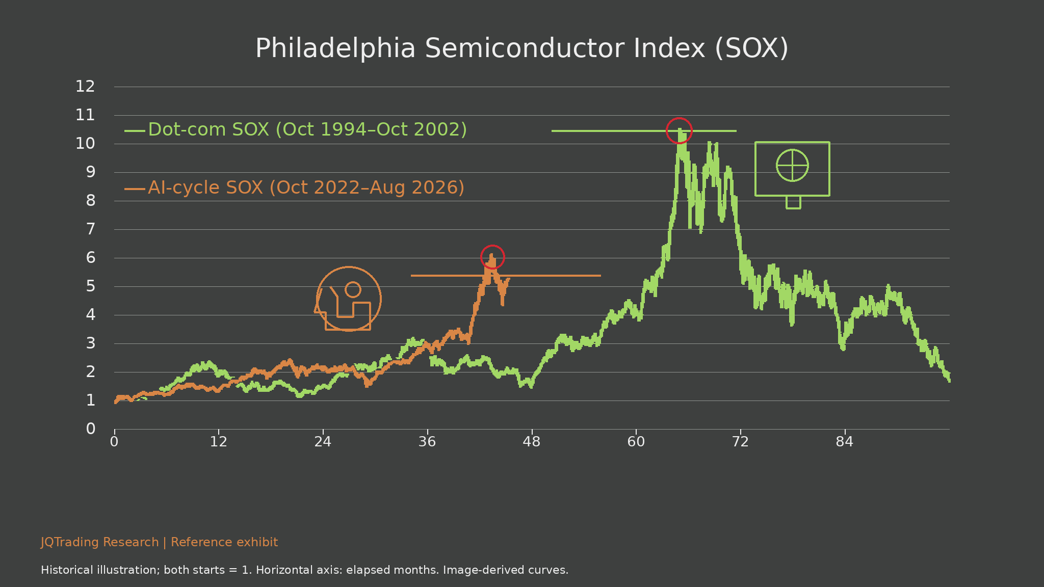
Starting the historical SOX cycle in October 1994 produces a reconstructed peak slightly above ten times its initial level. The AI series reaches roughly six times its initial level in June 2026. A purely mechanical comparison therefore leaves substantial apparent headroom.
Investment interpretation
Moving from six to roughly ten would imply about two-thirds additional appreciation; an almost-doubling narrative is only a loose historical extrapolation. More important, this result arises from the selected baseline. It is not an earnings-based valuation target.
Limits and monitoring
Both starts equal one and the horizontal axis measures months from the respective start. The historical series continues after its peak; the orange series stops at August 2026. Neither its shorter length nor its visual position predicts the missing future path.
Exhibit 08. Philadelphia Semiconductor Index (SOX)
What the exhibit shows
Starting the historical series in November 1996 reduces its subsequent peak multiple to around six. On this alignment the June 2026 AI peak looks close to the older cycle’s maximum, unlike the 1994 comparison.
Investment interpretation
The contrast between the two exhibits is the evidence: an apparently bullish or bearish conclusion can be created by changing the starting date. Initial valuation matters, but cannot by itself align different industrial structures, interest rates and business economics.
Limits and monitoring
A visual similarity is insufficient to establish that a top has occurred. Demand quality, utilization, rental yields and orders must confirm a deteriorating operating cycle. The October-versus-November 2022 baseline discrepancy also remains material for exact comparisons.
Exhibit 09. Three phases of the dot-com cycle
What the exhibit shows
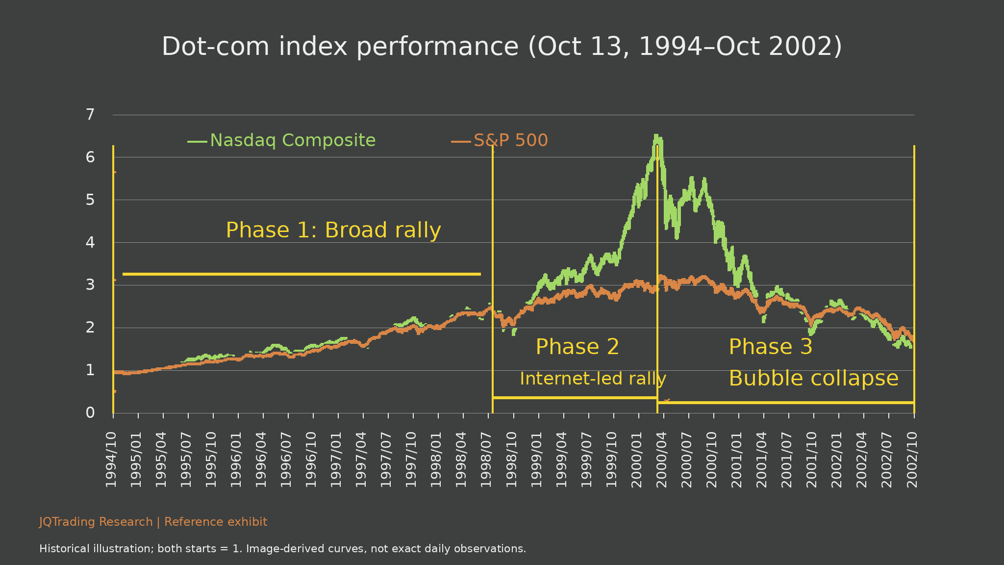
The normalized Nasdaq and S&P comparison divides the internet cycle into a broad rally, a more concentrated internet-led advance and a collapse. The concentrated phase can be further divided into applications leading first and hardware leading later.
Investment interpretation
A market can rise even while leadership becomes narrower or migrates upstream. Such rotation is economically relevant when customers commit capital faster than they earn returns from it. It is not a sufficient signal on its own because bottleneck suppliers can lead during healthy growth too.
Limits and monitoring
The phase boundaries are retrospective. They should not be treated as ex ante trading rules. The image-derived lines do not supply a daily backtest, and the company table that follows contains selected firms rather than the entire historical universe.
Exhibit 10. Dot-com company returns: Full table
What the exhibit shows
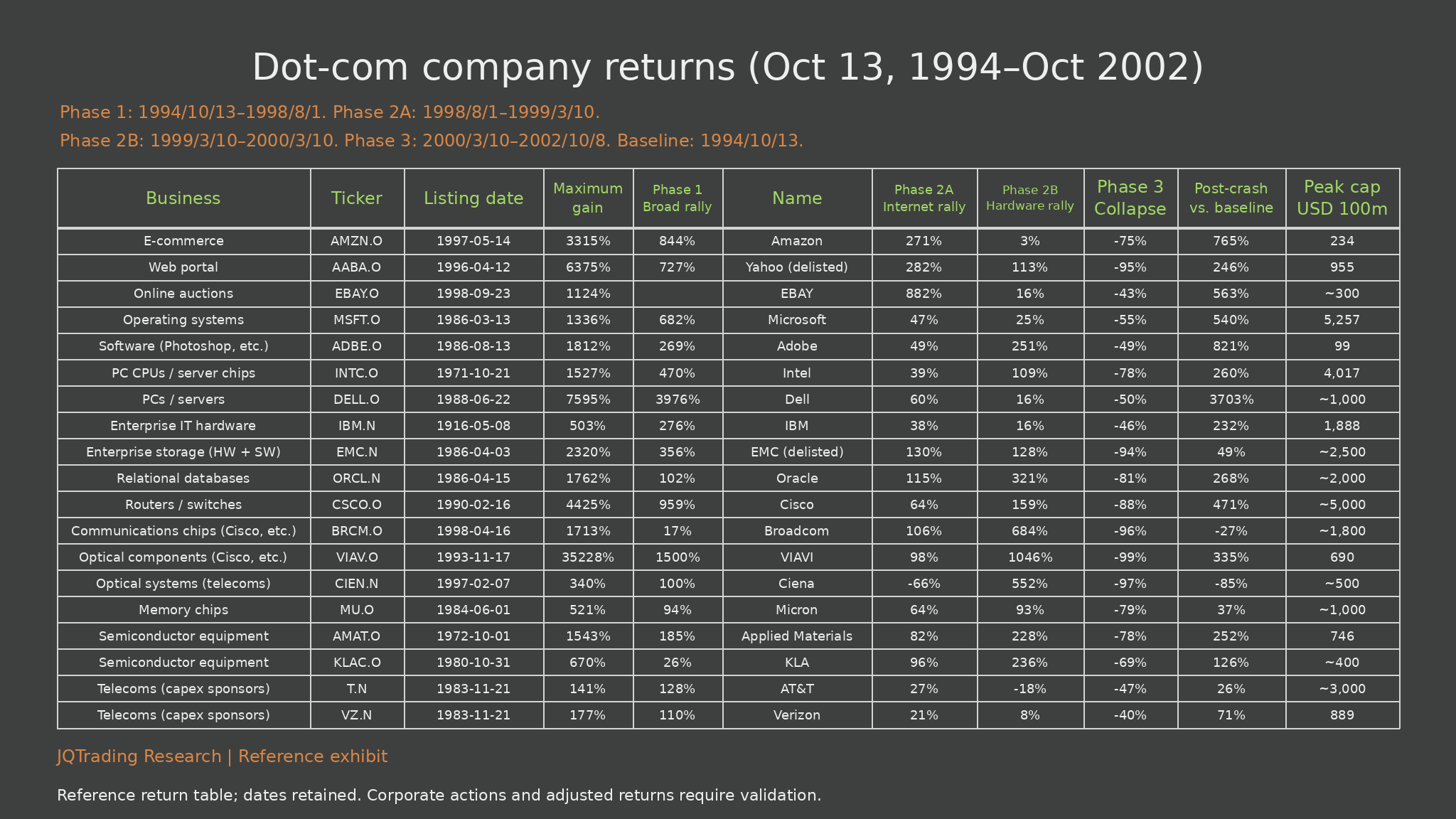
The full 19-company table retains business, ticker, listing date, maximum gain, broad-rally return, application-phase return, hardware-phase return, collapse return, post-crash comparison and peak capitalization in USD 100 million. Phase 1 is October 13, 1994-August 1, 1998; phase 2A runs to March 10, 1999; phase 2B to March 10, 2000; phase 3 ends October 8, 2002.
Investment interpretation
The table records Amazon, Yahoo and eBay at +271%, +282% and +882% during phase 2A. In phase 2B Amazon is +3% and eBay +16%, while Cisco is +159%, Broadcom +684%, VIAVI +1,046%, Applied Materials +228% and KLA +236%. AT&T is -18% and Verizon +8%. Selected hardware collapse entries run from KLA -69% to VIAVI -99%, illustrating how upstream leadership can reverse.
Limits and monitoring
All cells, blanks and approximate capitalization labels are retained. Returns are reference values, not newly validated adjusted series. Legacy tickers, predecessor businesses, delistings, spin-offs and dividends complicate interpretation; the post-crash-versus-baseline column should not be assumed to be a standard total-return measure.
4. Read the supply chain from the customer backward
The AI chain connects applications and users, model providers, cloud and compute services, accelerators and memory, foundries, and semiconductor equipment. Integrated businesses span multiple stages, so competitive strength and cyclical exposure must be evaluated separately for each activity.
Applications create the clearest evidence of final demand when customers renew because a product saves time, improves revenue or reduces errors. Model providers translate usage into revenue while managing serving costs. Compute operators monetize capacity. Chip, memory and equipment suppliers monetize the expansion needed to serve that usage.
A demand slowdown need not immediately appear in equipment revenue. Existing contracts, deployment schedules and backlog can delay the transmission. Conversely, constraints in power, packaging or memory may keep some suppliers strong even as another layer weakens. There is no universal lag length.
This makes the chain a monitoring framework rather than a mechanical countdown. Our strongest concern would arise when weaker renewal and paid usage coincide with falling rental yields, increasing spare capacity, softer hardware orders and deteriorating backlog quality.
The historical internet map helps explain why capital-spending sponsors and their suppliers can produce different returns. The AI map then identifies comparable economic roles, and the indicators table converts those roles into a monitoring framework. Software can often expand delivery faster than factories can expand production, which is why physical bottlenecks can create temporary scarcity profits.
Exhibit 11. Internet supply chain
What the exhibit shows
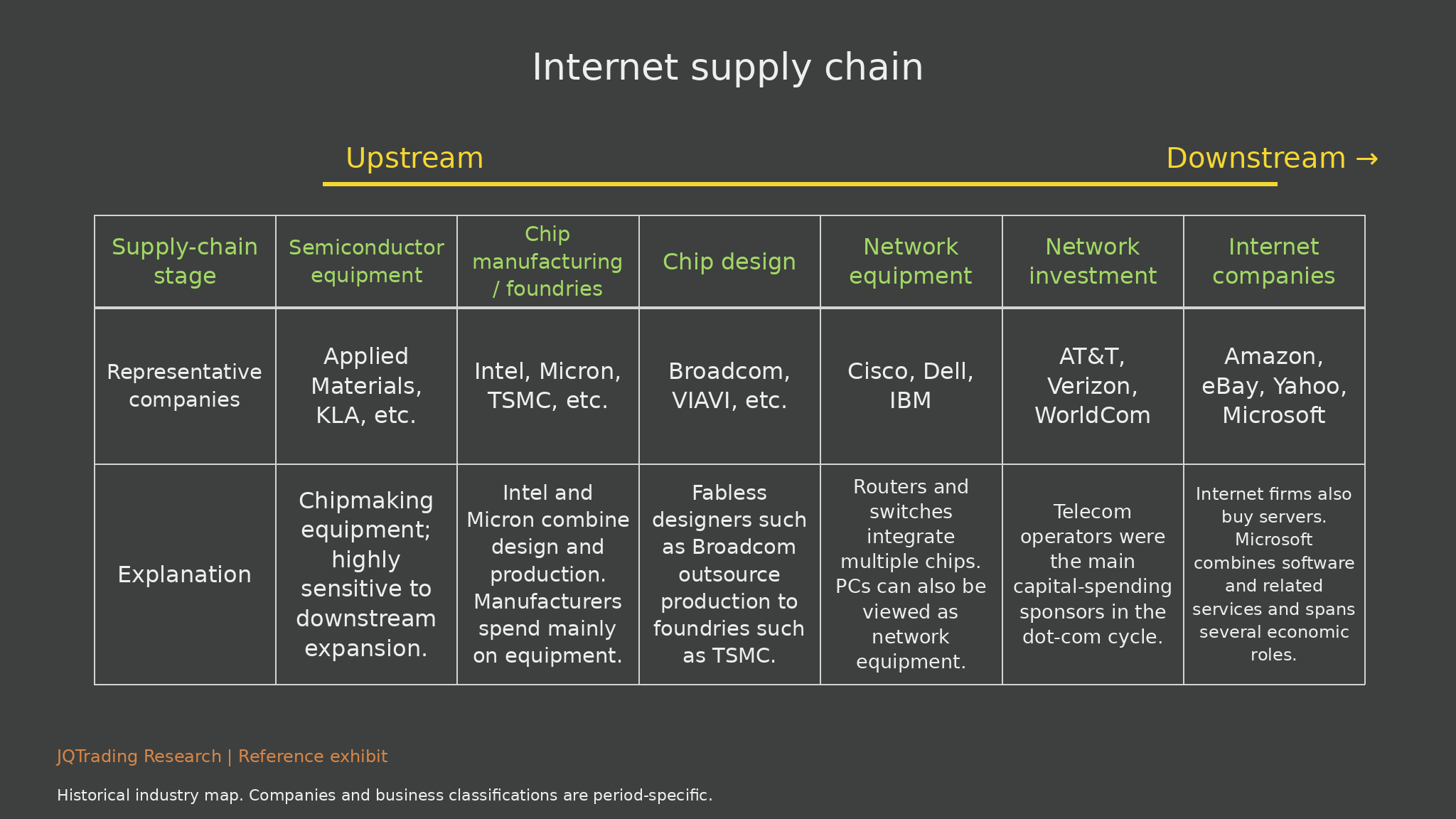
The historical map runs from equipment through chip manufacturing, chip design, network equipment, network investment and internet applications. It includes Applied Materials and KLA; Intel, Micron and TSMC; Broadcom and VIAVI; Cisco, Dell and IBM; telecom operators; and internet or software firms.
Investment interpretation
Telecom investment created orders for networks, chips and equipment before end-user economics necessarily justified the spending. Upstream suppliers could report strong revenue while the sponsors of that revenue faced weaker investor confidence. The analogous AI question concerns returns on cloud and model spending.
Limits and monitoring
The table is a simplified historical classification. Microsoft and integrated chip manufacturers do not fit a single stage cleanly. Organizational structure and business mix should be evaluated separately from the map.
Exhibit 12. AI supply chain
What the exhibit shows
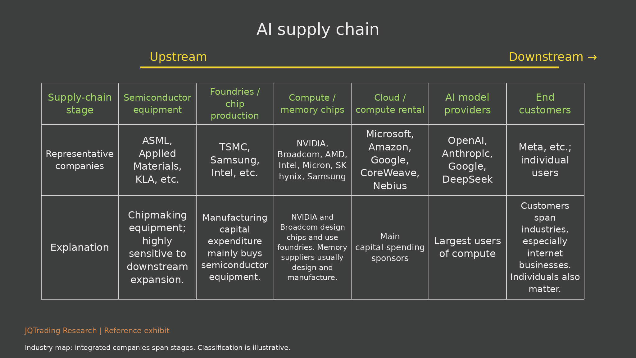
The full AI map identifies equipment; foundries and production; compute and memory; cloud and compute rental; model providers; and end customers. Representative names include ASML, TSMC, NVIDIA, Broadcom, AMD, Micron, SK hynix, Microsoft, Amazon, Google, CoreWeave, Nebius, OpenAI and Anthropic.
Investment interpretation
End customers fund the chain through useful applications, while model providers and cloud operators commit capacity ahead of realization. Integrated enterprises can combine final demand, internal models and their own infrastructure, so the apparent customer-supplier chain is not always linear.
Limits and monitoring
The map shows economic roles rather than a current exhaustive company list. Data-center power, networking, packaging and application distribution remain relevant even when not shown as separate columns.
Exhibit 13. AI supply chain and indicators
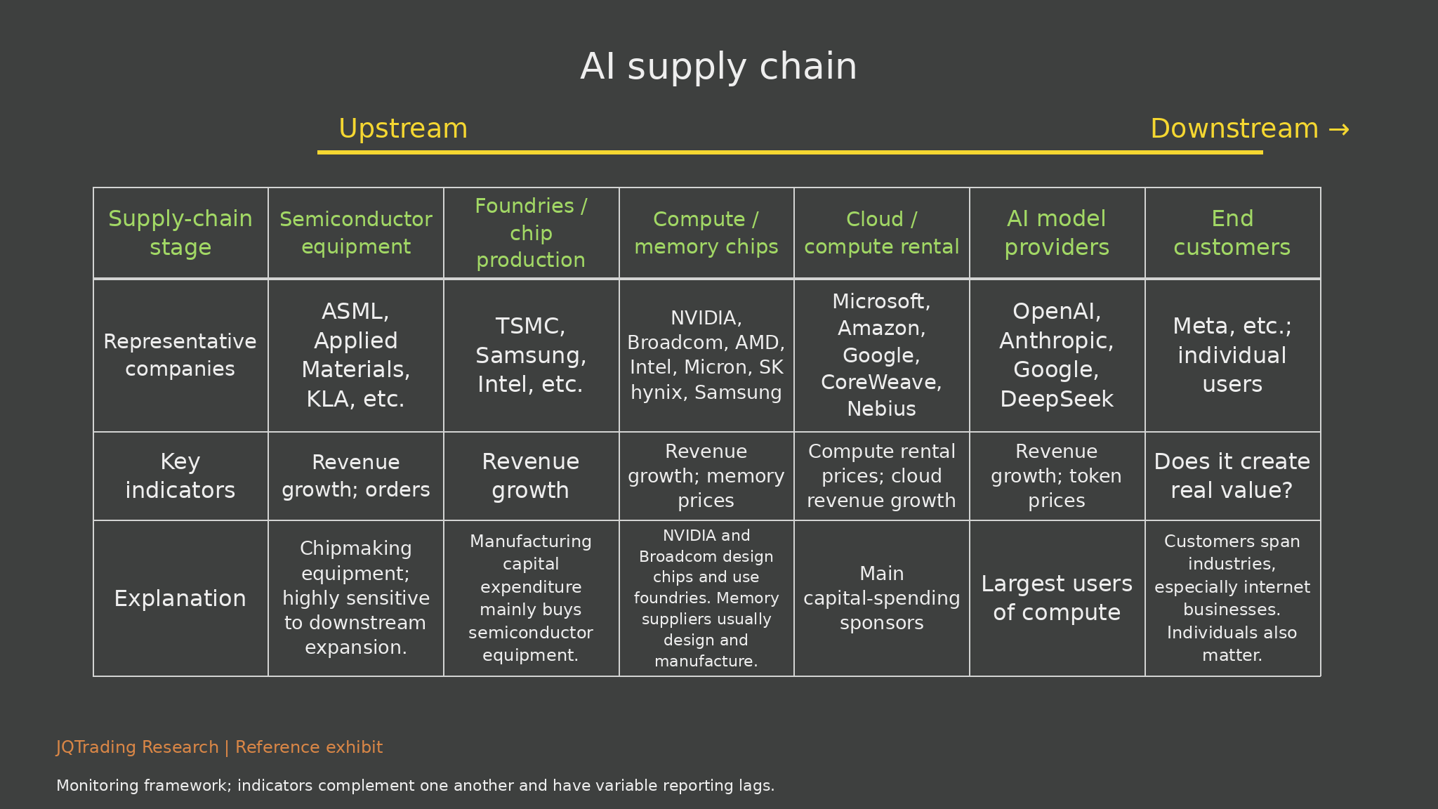
What the exhibit shows
The indicators progress from equipment orders and revenue, foundry revenue, chip revenue and memory prices, to rental prices and cloud growth, model growth and token pricing, and finally real customer value. Each stage has a different reporting cadence.
Investment interpretation
We start with customer outcomes and work backward. A weak model metric is more serious when falling compute yields and softer hardware orders confirm it. Conversely, improving task economics and strong paid renewals can make lower token prices a positive adoption signal.
Limits and monitoring
An early-looking metric can be distorted by discounts, mix, supply constraints or recognition rules. There is no fixed lag from model weakness to chip or equipment weakness. Monitor receivables, contract obligations and cancellations as well as reported growth.
Exhibit 14. Cash flow and indicators from users to equipment
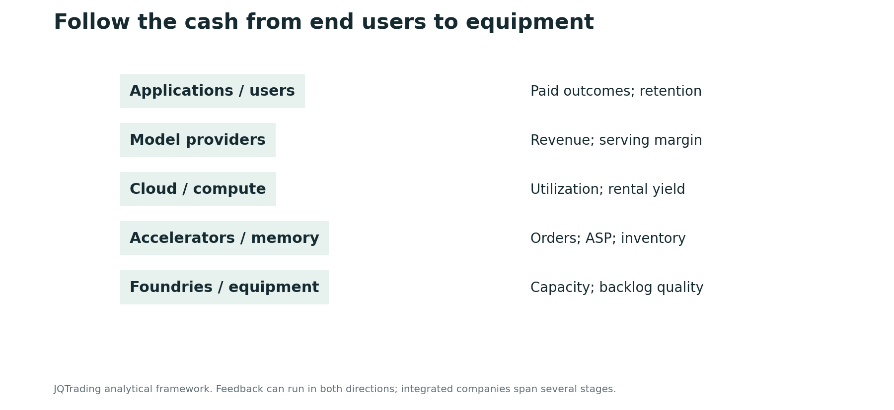
What the exhibit shows
This compact monitoring exhibit follows paid outcomes and retention at the user layer, revenue and serving margins at the model layer, utilization and rental yields at compute operators, orders and inventory at chips, and capacity and backlog quality at manufacturers.
Investment interpretation
It provides a repeatable dashboard for interpreting the more detailed supply-chain tables. The strongest adverse case is deterioration across several layers rather than a single falling share price or a isolated price cut.
Limits and monitoring
These are qualitative relationships, not measured coefficients or a forecast model. Internal transactions and vertically integrated businesses require care to avoid double counting.
5. Cheaper intelligence can expand usage and compress margins
AI inference carries a recurring compute cost. Traditional software and internet services also have operating costs; their marginal costs are not literally zero. The relevant question is whether each business can expand revenue faster than the costs needed to deliver additional useful work.
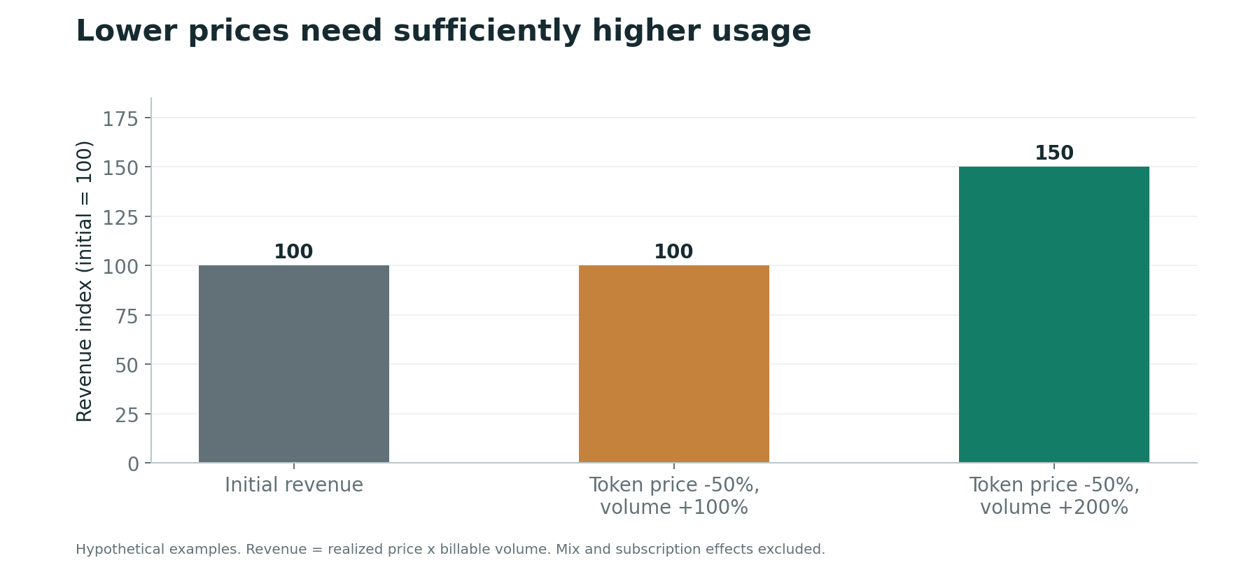
A 50% decline in realized price requires a doubling of billable volume merely to maintain revenue. Tripling volume raises revenue by 50%, before considering costs. Falling unit costs can make either case profitable, but the result depends on the pace of efficiency improvements, product mix and customer willingness to pay.
Token prices alone are an incomplete measure. Models differ in capability, latency, context, reasoning effort and reliability. Compare the total cost of completing a comparable task, including failed attempts and human review. A nominally cheaper token can still produce a more expensive workflow.
Competition among closed models, open-weight alternatives and request routers can reduce loyalty at the model layer. At the application layer, proprietary workflow integration, accumulated context, permissions, evaluation systems and distribution can create switching costs. Model providers can also build these strengths. Neither permanently weak retention nor a fixed mature net margin should be assumed.
The business-model matrix, routing diagram and full provider inventory add three separate tests: the cost of serving demand, the ability of customers to switch, and the financial endurance of competitors. We retain the original stylized assumptions while rejecting literal zero operating cost or a universal model cost percentage. Mature net margins near 10% belong in a sensitivity analysis, not a categorical prediction.
Exhibit 15. Software, internet and AI model business models
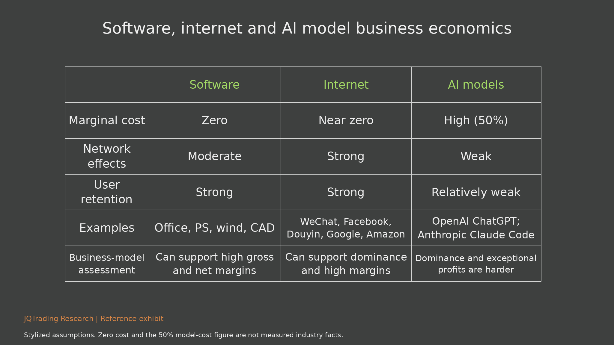
What the exhibit shows
The reference comparison assigns software low incremental delivery cost, internet platforms stronger network effects and model providers recurring compute expense. It also lists retention and familiar products. The original zero-cost labels and 50% model-cost assumption remain visible for completeness.
Investment interpretation
Office, Photoshop and engineering software can benefit from learned workflows; social and marketplace platforms can benefit from networks. Model switching may be easier when capabilities converge, but enterprise integration, context, brand and distribution can still support durable retention. The quality of these advantages differs by product.
Limits and monitoring
Zero marginal cost is an approximation, not an accounting fact. The 50% cost assumption is unverified and cannot establish gross or net margins. A conjectured 10% mature model net margin is a sensitivity case, not an industry forecast.
Exhibit 16. Developers route requests through a model aggregator
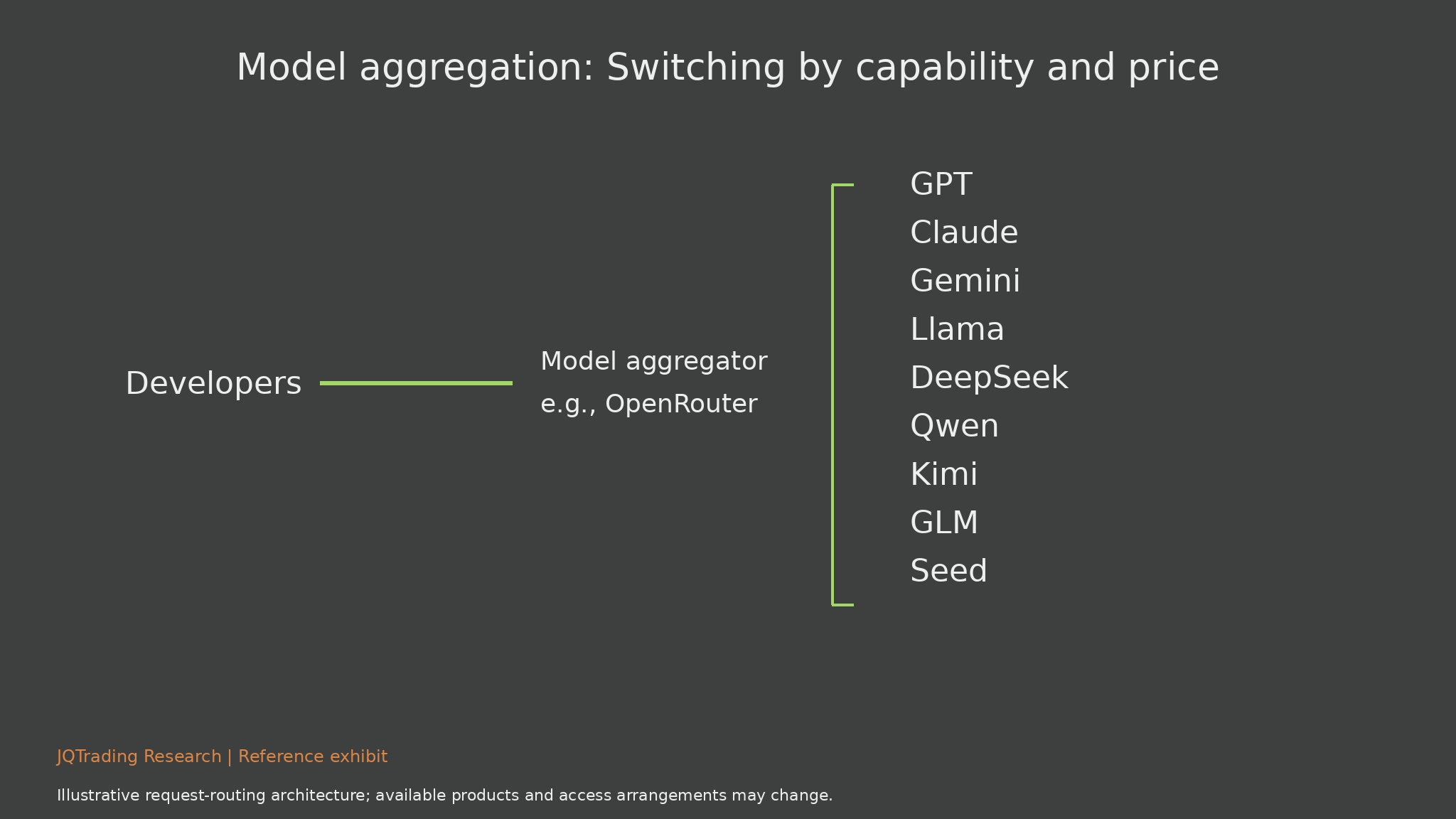
What the exhibit shows
The architecture routes developer requests through an aggregator to different model families, including GPT, Claude, Gemini, Llama, DeepSeek, Qwen, Kimi, GLM and Seed. The route can depend on price, capability, latency or availability.
Investment interpretation
Aggregation can weaken dependence on a single underlying model and transfer some customer relationship to the application or routing layer. This may increase price competition, while creating value for reliable evaluation, fallback and deployment tools.
Limits and monitoring
Switching is not frictionless. Data governance, tool formats, evaluation, model behavior and enterprise approval can add substantial cost. The diagram does not establish availability of every listed family on every service at every date.
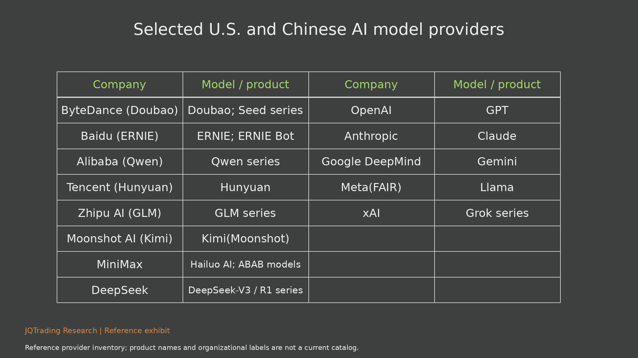
Exhibit 17. U.S. and Chinese AI model providers: Full table
What the exhibit shows
The provider table retains ByteDance/Doubao, Baidu/ERNIE, Alibaba/Qwen, Tencent/Hunyuan, Zhipu/GLM, Moonshot/Kimi, MiniMax and DeepSeek, alongside OpenAI/GPT, Anthropic/Claude, Google/Gemini, Meta/Llama and xAI/Grok.
Investment interpretation
Competition includes independent model companies and platforms with established distribution and profitable core businesses. Capability leadership can change, and financial endurance may matter as much as a benchmark lead. Model-only firms are more exposed if funding weakens before recurring gross profit covers investment.
Limits and monitoring
The inventory is dated and product labels are preserved, not verified as an up-to-date catalog. Listing a provider does not quantify market share, technical parity or the probability that its product survives.
Exhibit 18. Price-volume sensitivity at the model layer
What the exhibit shows
With initial revenue indexed to 100, a 50% realized-price decline and a 100% volume increase leave revenue at 100. The same price decline and a 200% volume increase produce revenue of 150.
Investment interpretation
Lower prices can democratize adoption, but suppliers need sufficient volume or lower serving cost to improve earnings. Agents may generate more tokens per workflow, so measured token growth must be reconciled with useful customer outcomes.
Limits and monitoring
The examples exclude subscription behavior and mix changes. They say nothing about actual company elasticity or cost efficiency. Compare equivalent tasks and reliability before treating price declines as either distress or progress.
6. Training and inference create different competitive tests
Frontier training places heavy demands on accelerator scale, software tooling, interconnects and distributed-system reliability. A strong ecosystem can make a hardware platform valuable beyond the chip’s standalone specifications. But even a durable moat does not eliminate sensitivity to customer budgets or the valuation paid for future growth.
Inference creates a broader optimization problem: throughput, memory capacity and bandwidth, latency, energy use, model compatibility and total cost per successful task. Alternative accelerators and cloud-designed chips can compete where workloads are sufficiently standardized. This does not make inference easy or remove the engineering value of software and networking.
The relevant competitive landscape includes general-purpose GPUs, custom cloud silicon and specialized accelerators, as well as domestic suppliers in China. A long supplier list demonstrates alternatives, not equivalent performance or immediate production readiness. Product announcements must be separated from shipped volume and proven customer economics.
For equipment and foundries, barriers in manufacturing and process technology may remain durable while order growth becomes cyclical. For memory, technical qualification and high-bandwidth requirements can support differentiated economics, but aggregate supply responses still matter. We prefer segment-level evidence to declaring every upstream company either a monopoly or a commodity.
The supplier inventory includes cloud companies that develop accelerators for internal use and independent firms seeking external customers. A chip announcement is not equivalent to qualified deployment. Procurement risk depends on software, system performance and availability as well as hardware specifications. Optical modules, packaging and testing can share the capex cycle, but their competitive strength also needs company-specific evaluation.
| Layer | Potential protection | Evidence to demand |
|---|---|---|
| Training platforms | Software ecosystem; scale reliability | Customer retention; system performance |
| Inference platforms | Cost, latency and integration | Cost per completed task; real deployment |
| Foundries and equipment | Process capability; qualification | Yield; utilization; order quality |
| Memory | Qualification; bandwidth; packaging | Contract economics; inventory; supply response |
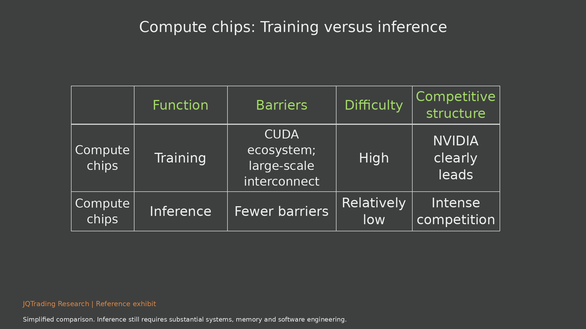
Exhibit 19. Training versus inference: Competitive barriers
What the exhibit shows
The training/inference matrix emphasizes training software and interconnect barriers, then presents inference as relatively more open to competition. Training can require highly coordinated large clusters; inference optimizes deployed tasks under service constraints.
Investment interpretation
CUDA, tooling, reliability and system-scale integration can protect a platform. Inference competition may favor different hardware for different workload shapes. A house-design versus house-construction analogy is useful intuition, but actual inference systems still require sophisticated engineering.
Limits and monitoring
The original description of inference as relatively low difficulty is a simplification. Memory, networking, latency, power and compatibility remain barriers. No benchmark or cost superiority is established by this table.
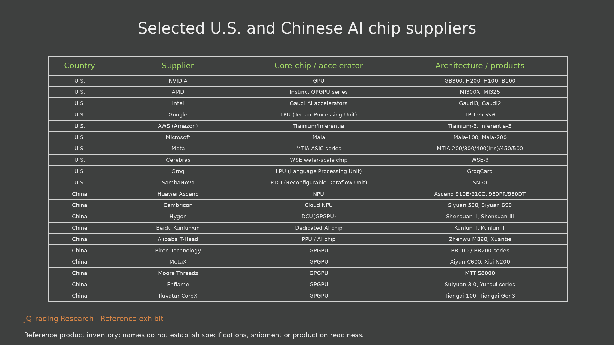
Exhibit 20. U.S. and Chinese AI chip suppliers: Full table
What the exhibit shows
The 20-supplier inventory retains ten U.S. entries and ten Chinese entries. It covers NVIDIA and AMD GPUs; Intel Gaudi; Google TPU; AWS Trainium/Inferentia; Microsoft Maia; Meta MTIA; Cerebras, Groq and SambaNova; and Huawei, Cambricon, Hygon, Kunlunxin, T-Head, Biren, MetaX, Moore Threads, Enflame and Iluvatar CoreX.
Investment interpretation
Cloud-designed chips can capture internal workloads without becoming a separately listed investment. Independent vendors need performance, software support, customer qualification and funding. A supply glut would expose differences between a competitive complete platform and a chip that benefits mainly from scarcity.
Limits and monitoring
All reference product names are retained, including generation labels. They are not validated specifications or evidence of mass production. Internal use, availability, export restrictions, entity changes and commercial status require separate verification.
7. Memory scarcity is powerful, but cyclical
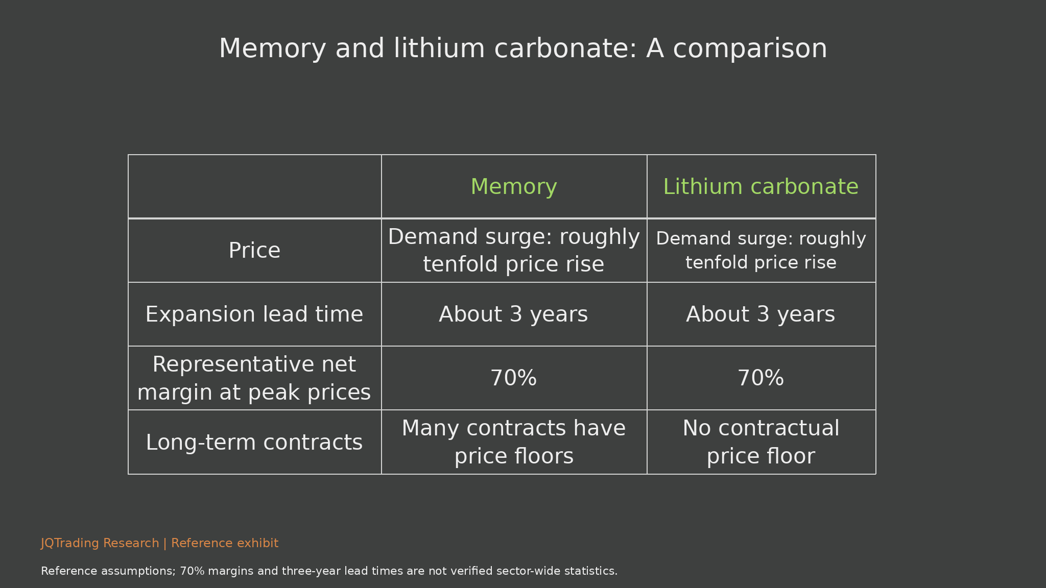
The memory-price and lithium-cycle comparisons illustrate an important capital-cycle risk: when supply cannot respond quickly, a demand shock raises prices and magnifies profits. High margins then encourage investment. Capacity arriving later can undermine the economics that justified the expansion.
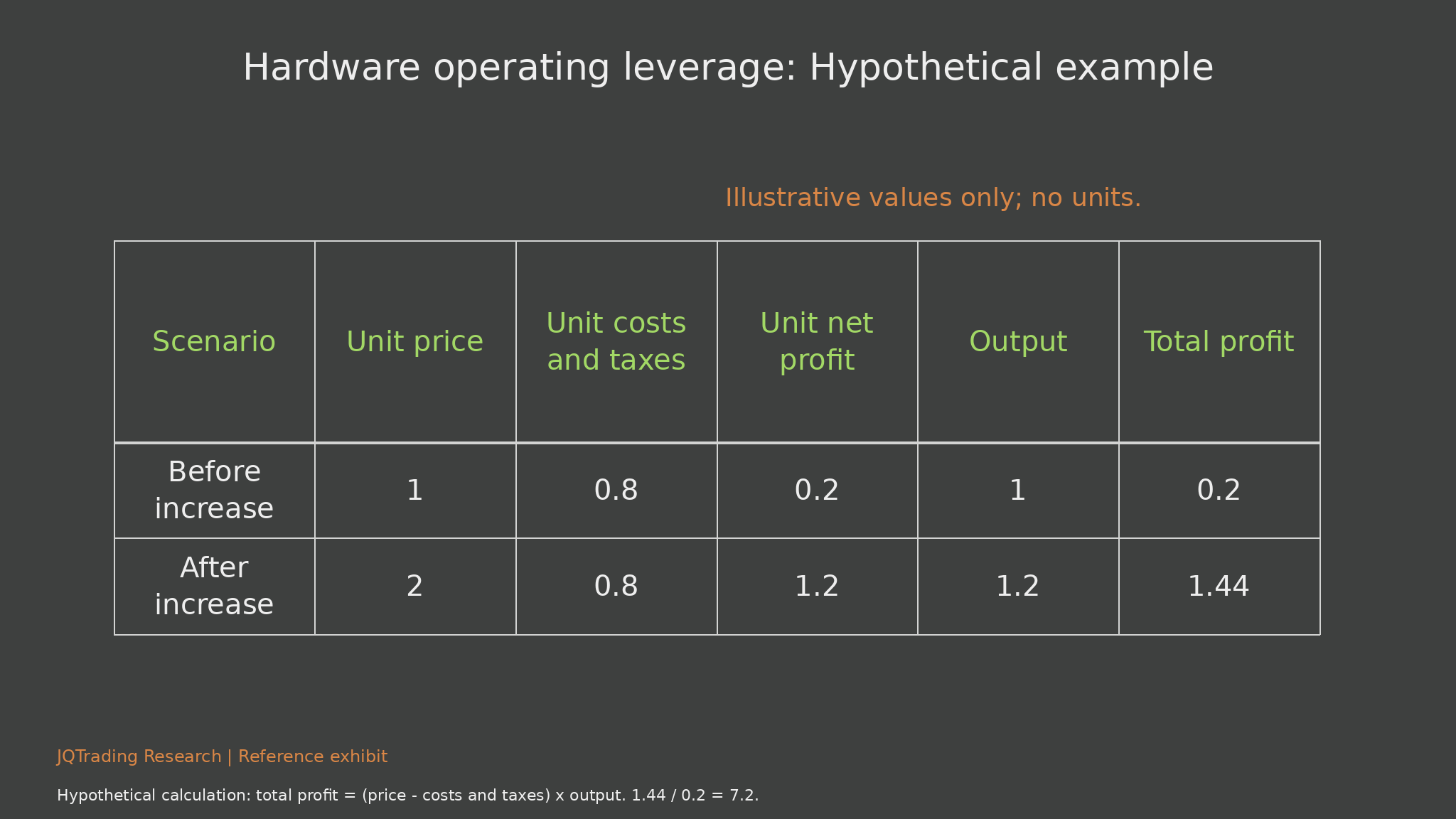
The illustrative calculation below holds unit cost and taxes at 0.8. Raising the selling price from 1 to 2 increases unit profit from 0.2 to 1.2. With output rising from 1 to 1.2, total profit rises from 0.2 to 1.44, or 7.2 times. The same sensitivity operates in reverse when prices normalize.
This is a teaching example, not a forecast of Micron or any supplier’s accounts. Real costs, product mix, yields, depreciation and taxes change. DDR5 spot prices do not represent all DRAM, NAND or HBM contracts. A lithium spot-price cycle cannot establish a memory company’s sustainable net margin.
Long-term contracts may improve visibility. Their protection depends on enforceable prices, volumes, duration, renegotiation rights and customer credit. A contractual floor is not a permanent industry price floor. We value cyclical suppliers using normalized earnings, supply growth and balance-sheet resilience, rather than applying a growth multiple to peak margins.
The full reference memory and lithium exhibits preserve their quoted points and contract assumptions so the capital-cycle argument remains visible. Their numerical limitations are also explicit. No unverified 70% peak margin or common three-year expansion period is used as a sector-wide forecast; normalized earnings and enforceable contract terms matter more than a selected peak.
Exhibit 21. Hardware profit sensitivity: Hypothetical example
What the exhibit shows
The table assumes unit price 1, unit costs and taxes 0.8, output 1 and total profit 0.2. Raising price to 2 with the same unit cost and output 1.2 produces total profit 1.44, or 7.2 times the original.
Investment interpretation
Hardware supply constraints can turn a moderate volume increase and scarcity pricing into much faster earnings growth. The same mechanism makes valuation based on peak profit dangerous: a reversal in price can compress profit faster than revenue.
Limits and monitoring
All values are unitless assumptions. Actual semiconductor suppliers have changing costs, yields, depreciation, mix and taxes. The calculation establishes operating sensitivity, not a specific future margin.
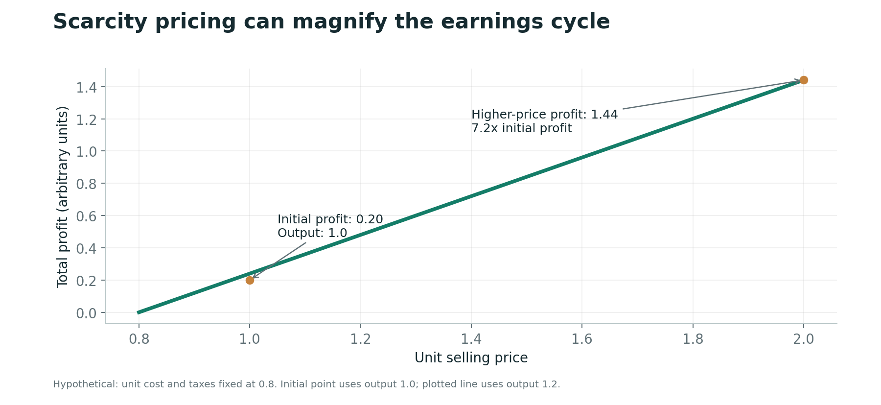
Exhibit 22. Scarcity pricing and operating leverage
What the exhibit shows
The plotted line shows profit sensitivity with output held at 1.2, while the initial point uses output 1.0. The endpoint at price 2 has total profit 1.44; the initial point at price 1 has total profit 0.2.
Investment interpretation
This visual makes the amplification in the preceding table easier to see. Investors should separate profits created by temporary prices from profits supported by durable production or product improvements.
Limits and monitoring
The initial point is intentionally off the constant-output curve. Cost and tax assumptions stay fixed for illustration; the chart is not a company earnings model.
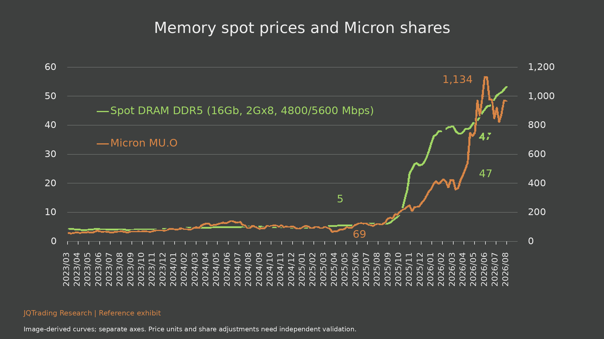
Exhibit 23. DDR5 spot prices and Micron shares
What the exhibit shows
The green DDR5 spot-price line and orange Micron share-price line use separate axes. The reference marks memory near 5 and 47 and the equity series near 69 and 1,134. The window runs from March 2023 to August 2026, with a steep late-cycle increase and an equity pullback.
Investment interpretation
The reference narrative describes an almost-tenfold memory-price move and a much larger equity advance. The economic point is scarcity and forward-looking repricing: shares can reverse before the commodity or component price reaches its peak. DDR5, HBM and NAND economics must still be analyzed separately.
Limits and monitoring
Price units, quotation conventions and stock adjustments have not been established for these labels. The 1,134 equity annotation must not be treated as a verified USD share price. The curve supports a qualitative comparison, not a precise valuation or return calculation.
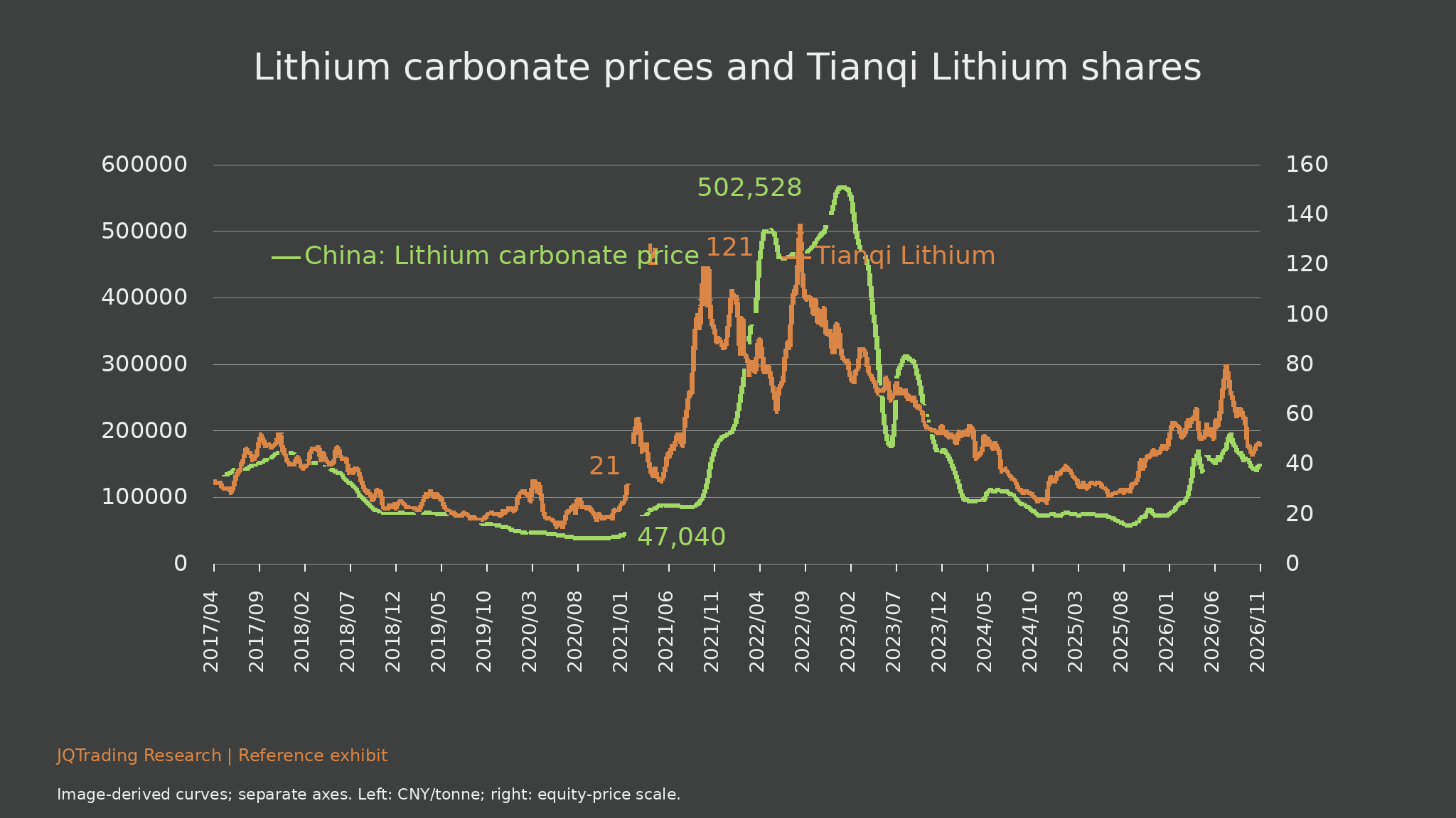
Exhibit 24. Lithium carbonate and Tianqi Lithium
What the exhibit shows
The lithium carbonate series is labeled in CNY per tonne, with annotations around 47,040 and 502,528. Tianqi’s separate equity-price scale includes reference points near 21 and 121. The chart covers April 2017-June 2026.
Investment interpretation
High input prices can encourage substantial capacity investment, followed by oversupply. Equities may anticipate that supply response before spot prices decline. This provides a capital-cycle analogy for memory, while acknowledging different manufacturing, qualification and end-market conditions.
Limits and monitoring
The curve is image-derived and the two axes have different units. The roughly 80% stock-loss narrative is not a newly computed adjusted total return. Lithium’s cycle does not establish memory’s expansion timing, contract protection or terminal margins.
Exhibit 25. Memory versus lithium carbonate
What the exhibit shows
The comparison retains reference assumptions of roughly tenfold price increases, about three years to expand capacity, representative 70% peak net margins, and greater contractual price protection in memory than lithium.
Investment interpretation
The general capital-cycle logic is useful: scarcity attracts capital, and delayed capacity can impair future returns. Long-term contracts can moderate exposure when their terms and counterparties remain enforceable. Contracts cannot make industry pricing permanently independent of supply.
Limits and monitoring
These numerical and contractual generalizations are unverified. A 70% margin is not accepted as a sector statistic, and a 20% normalized memory margin is only a proposed sensitivity. Expansion timing and floor protection must be validated supplier by supplier.
8. Watch the sequence, and test competing explanations
The bearish transmission scenario starts with weaker end-user economics: slower paid adoption, poorer renewals or pressure on realized prices. If serving efficiencies fail to compensate, model margins deteriorate and financing becomes more difficult. Unused compute can then increase, weakening rental yields and eventually reducing hardware and equipment orders.
Several links can break this sequence. Demand may be constrained by capacity rather than willingness to pay. Better models may unlock new tasks. Cheaper inference can make previously uneconomic workloads viable. Capacity released by one operator may be absorbed by another. These alternatives require evidence, not optimism by default.
Likewise, one falling token price is not proof of distress, one order cut is not an industry collapse, and one revenue acceleration is not proof of healthy returns. We seek convergence across indicators, track the definitions consistently, and distinguish commitments from delivered capacity.
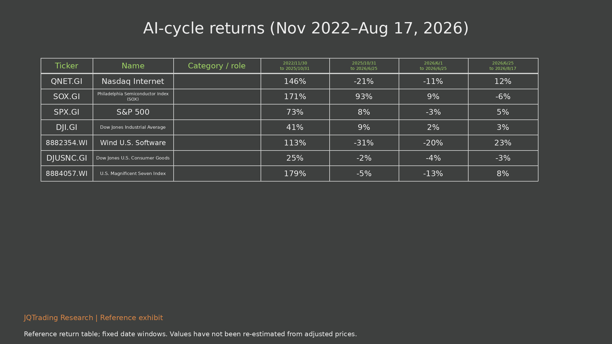
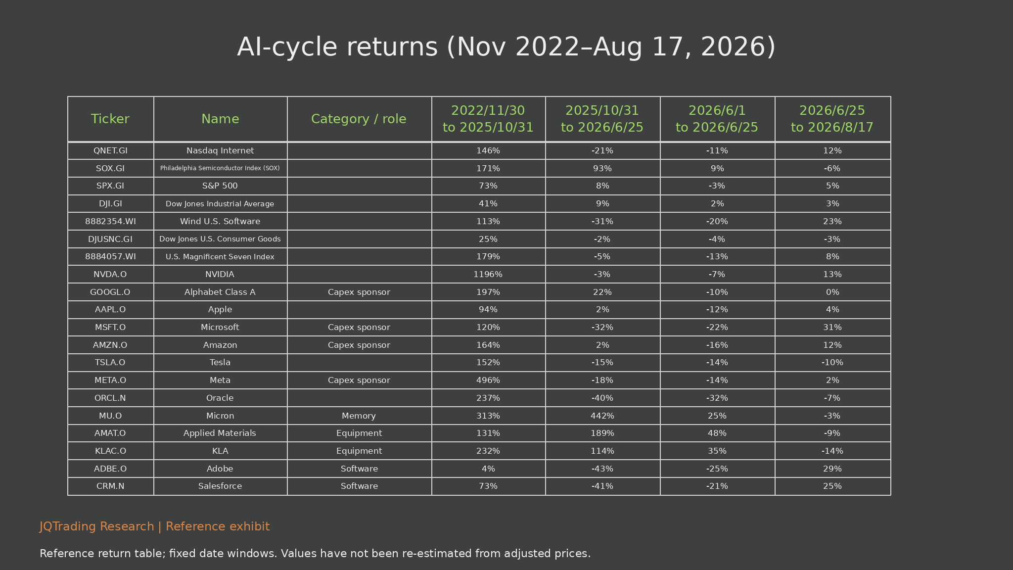
The two return tables document the proposed market signal in four fixed windows, including the late-June reversal. They distinguish sponsors, software and upstream suppliers without assuming that one group behaves uniformly. A slowdown in model growth and pressure on realized prices may be earlier signals; rental yields, utilization and supplier orders offer operating confirmation.
| Signal | Healthy interpretation | Adverse interpretation |
|---|---|---|
| Lower task price | Efficiency gains with stable margins | Discounting with margin compression |
| More compute capacity | Deployment absorbs incremental supply | Utilization and rental yield fall |
| Model revenue growth | Renewing customers expand paid use | Credits or partner concentration dominate |
| Hardware backlog | Firm orders with healthy delivery | Deferrals, cancellations or receivable stress |
| Rising supplier margin | Durable mix and productivity gains | Temporary scarcity pricing |
Exhibit 26. AI-cycle company and index returns (indices)
What the exhibit shows
For November 30, 2022-October 31, 2025, the reference index table shows internet +146%, SOX +171%, S&P 500 +73%, software +113% and the Magnificent Seven +179%. For October 31, 2025-June 25, 2026, SOX is +93%, internet -21%, software -31% and the Magnificent Seven -5%.
Investment interpretation
The selected windows suggest leadership shifting from broad AI participation toward hardware. This may reflect doubts about returns on customer spending, stronger upstream scarcity economics, software substitution concerns or different entry valuations. Price performance alone cannot distinguish these explanations.
Limits and monitoring
The June 1-June 25 window overlaps the longer October-June window. The columns are not four independent phases, and returns must not be added. The fixed-date values are retained, not recalculated from adjusted histories.
Exhibit 27. AI-cycle company and index returns (full table)
What the exhibit shows
The full table preserves all 20 index and company rows across four date windows. In October 2025-June 2026, Micron is +442%, Applied Materials +189% and KLA +114%, while Microsoft is -32%, Meta -18%, Oracle -40%, Adobe -43% and Salesforce -41%. Alphabet is +22% and Amazon +2%, demonstrating that sponsors are not uniformly weak.
Investment interpretation
The late-June-August window records Microsoft +31%, Amazon +12%, Adobe +29% and Salesforce +25%, alongside Micron -3%, Applied Materials -9% and KLA -14%. This partial reversal cautions against extrapolating divergence indefinitely. Later hardware weakness can coexist with better application or cloud expectations.
Limits and monitoring
NVIDIA’s early +1,196% reference return and all remaining cells are preserved in the table. Dates, classifications and adjustment conventions must be checked before using these values for trading. Share-price weakness can influence financing incentives but does not mechanically determine corporate capex.
9. Good businesses can still be expensive securities
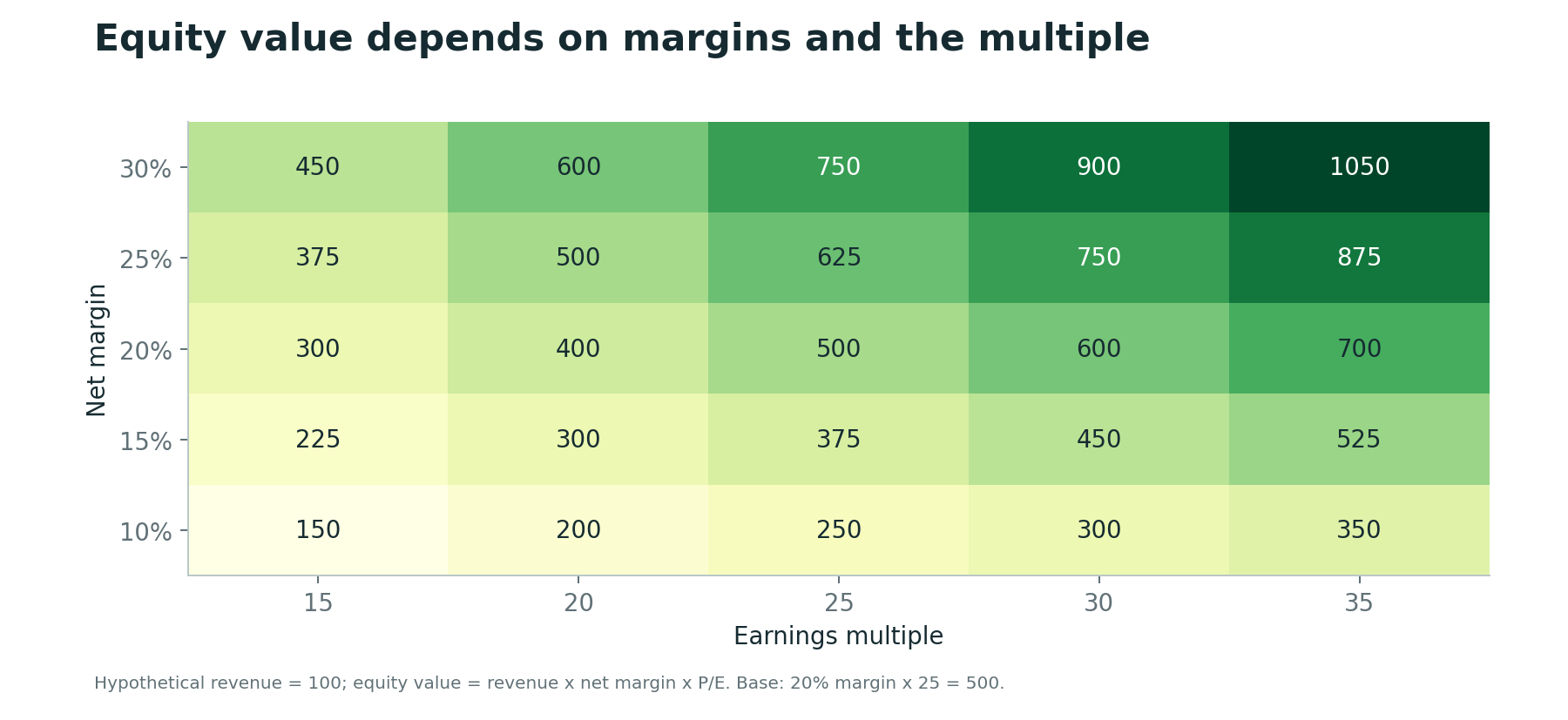
A simple sensitivity model makes the distinction visible. With revenue fixed at 100, a 20% net margin and a 25-times earnings multiple imply equity value of 500. At a 10% margin and 20-times multiple, the value becomes 200: a 60% decline despite unchanged revenue. At a 25% margin and 30-times multiple, value rises to 750.
These are illustrative arithmetic outcomes, not stock targets or assigned probabilities. Real valuation must incorporate growth, dilution, net debt, cash flow, capital intensity and the appropriate valuation method. Price-to-earnings multiples are especially unreliable for loss-making companies and suppliers earning abnormal peak profits.
A perceived moat supports the durability of earnings. It does not tell us how much future success is already in the price. The most demanding valuations need both favorable earnings and continued willingness to pay a premium. Rising discount rates or a lower terminal margin can offset substantial business growth.
Our investment discipline is to specify the earnings required to justify a price, then compare those requirements with utilization, renewals, margins and capital needs. We do not assign a universal 50% or 70% drawdown to an entire supply-chain category.
The complete risk discussion is therefore two-dimensional: how resilient is the business, and how demanding is the price? A monopoly-like position can soften margin erosion but still leave substantial multiple compression. Company and portfolio risk should be modeled explicitly rather than inferred from a single historical category drawdown.
Exhibit 28. Equity-value sensitivity to margins and the multiple
What the exhibit shows
With revenue fixed at 100, a 20% net margin and 25-times P/E imply equity value 500. At 10% and 20 times, value is 200; at 25% and 30 times, it is 750. The matrix displays the complete combinations from 10%-30% margin and 15-35 times earnings.
Investment interpretation
A 60% hypothetical value decline can occur without falling revenue. This separates a bullish adoption thesis from a bullish entry-price thesis. Moats improve the probability of durable earnings but do not protect investors from paying too much for them.
Limits and monitoring
These are arithmetic sensitivities, not price targets. Net debt, dilution, reinvestment and discount rates are excluded. P/E is unsuitable for some loss-making businesses and can flatter suppliers at peak-cycle profit.
10. Employment is an adoption question and a demand question
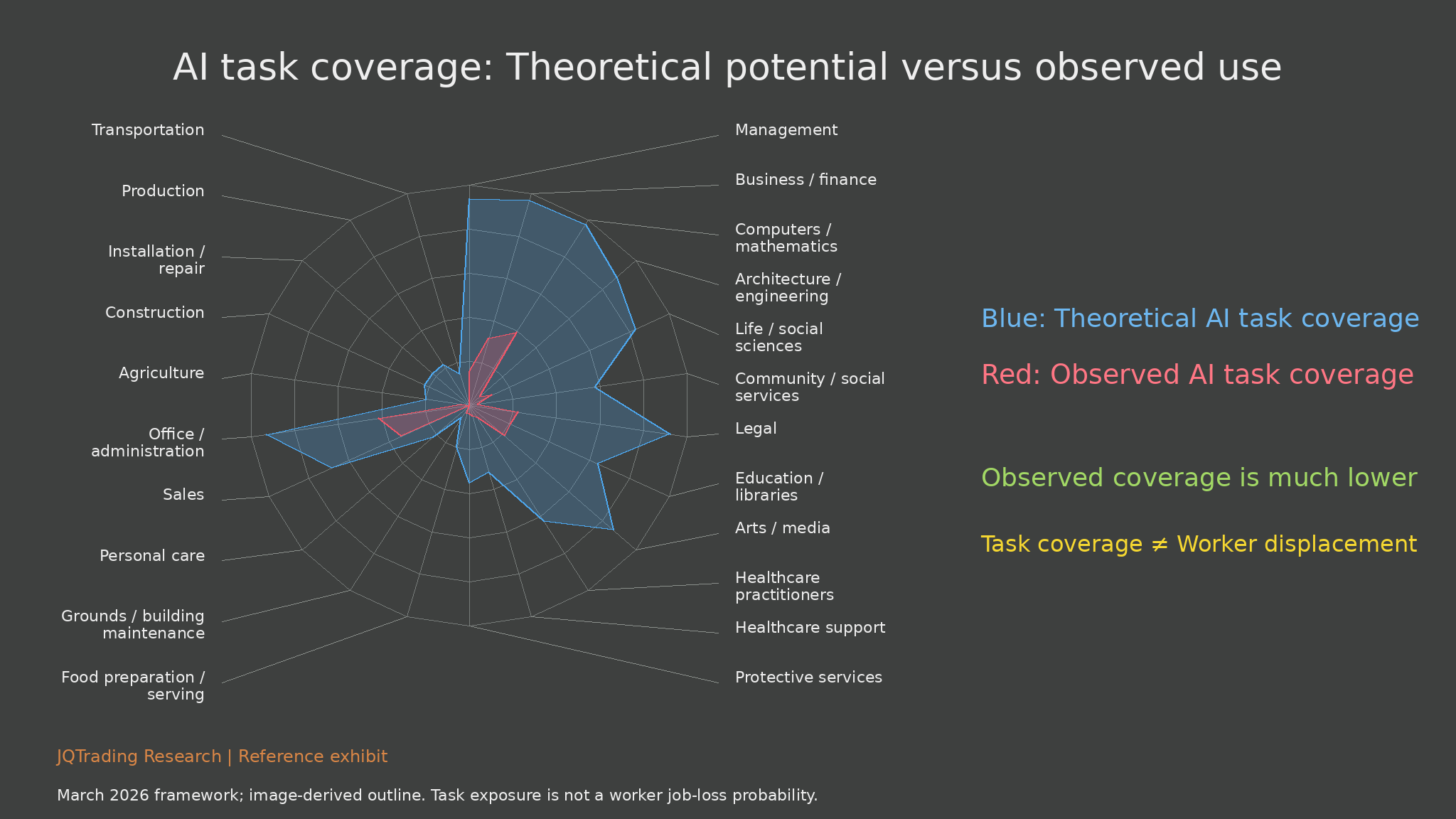
Task exposure should not be confused with job elimination. The March 2026 labor-market study found a substantial gap between theoretically feasible AI use and observed use. It reported no systematic rise in unemployment among highly exposed workers since late 2022, while finding suggestive evidence of slower hiring among younger workers in exposed occupations. These are dated findings, not a claim about all labor-market outcomes today.
The exposure radar is therefore best understood as a map of potential workflow change. A task can be accelerated without an entire occupation disappearing. Reliability, responsibility, regulation and organizational redesign influence whether technical capability becomes actual substitution.
For the long-term outlook, adoption must cross the distance between demonstrations and trusted production. Human oversight and integration costs can reduce savings initially. If these barriers fall, productivity and output can improve, creating new markets and reducing costs.
The macroeconomic effect also depends on how gains are distributed. Concentrated income gains could weaken demand in some sectors; new jobs, lower prices, investment and policy responses could offset that pressure. A productivity shock does not mechanically imply either a boom or a crisis. We monitor hiring, wages, consumption and adoption together.
The full radar adds occupational detail to the economic outlook. Productivity expands supply, while household income, prices, new occupations and policy affect demand. Robotics could extend exposure to physical work, but requires additional deployment and capital. Neither broad inequality nor a repeat of the Great Depression follows mechanically from present task-exposure measures.
| Measure | What it tells investors | What it does not establish |
|---|---|---|
| Theoretical task exposure | Potential technical reach | Probability of losing a job |
| Observed AI use | Current adoption in sampled workflows | Economy-wide causal impact |
| Hiring and wages | Adjustment in labor demand | AI as the sole cause |
| Realized productivity | Value from deployment | Equal gains across firms or workers |
Exhibit 29. Occupational task coverage: Radar chart
What the exhibit shows
The 22-category radar contrasts theoretical task exposure in blue with observed use in red. It covers management, finance, computing, engineering, science, social services, legal, education, media, healthcare, protective services, food, maintenance, personal care, sales, administration, agriculture, construction, repair, production and transport.
Investment interpretation
The wide gap suggests technical possibility is ahead of workplace deployment. Rough readings near 80% theoretical exposure in some knowledge-work categories and around 30% observed computing exposure are indicative only. Adoption, integration and reliability therefore shape the size and timing of economic effects.
Limits and monitoring
The outline is image-derived and exact category values are unavailable. Task exposure is not the fraction of workers who will lose jobs. The March study reported no systematic unemployment increase in highly exposed occupations since late 2022, while suggesting weaker hiring for younger workers; these are dated findings.
11. Three scenarios for the next investment phase
Our base case is that AI becomes more useful and more widely deployed, while investment returns diverge sharply. Price competition and capacity growth put pressure on weaker operators. Businesses with distribution, workflow integration and financing flexibility can gain share without every infrastructure supplier sustaining peak margins.
The bull case requires more than impressive benchmarks. Reliable agents, stronger renewal rates and rising paid usage would need to turn lower costs into broader profitable demand. Utilization stays healthy, customer returns improve and cash generation increasingly finances expansion.
The bear case combines weaker incremental demand with rigid commitments. Model economics deteriorate, external funding tightens, rental yields decline and hardware orders weaken. Share prices may adjust before the worst accounting results. The long-term usefulness of AI can remain intact throughout this correction.
We assign no numerical probabilities because the available evidence does not support that precision. The monitoring signals below determine whether the stance should become more constructive or more defensive.
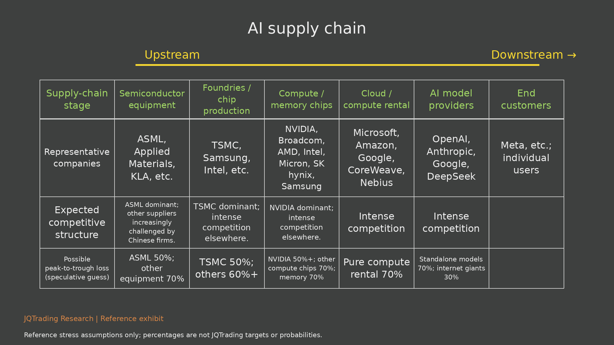
The reference drawdown matrix is included below as a stress discussion, preserving every sector estimate and the associated competitive-structure judgments. We do not convert it into investment targets. Its proper use is to identify which financial assumptions need testing under each scenario, alongside customer renewal, utilization, financing and order indicators.
| Scenario | Operating pattern | Investment implication |
|---|---|---|
| Bull: productive scale | Strong renewal; improving unit margin; high utilization | Broader earnings participation; test entry valuation |
| Base: adoption with dispersion | Usage rises; competition and capex absorb value | Select durable cash generators and differentiated suppliers |
| Bear: capacity exceeds paid demand | Weak renewals; lower rental yields; order deferrals | Reduce exposure to leverage and peak earnings |
Exhibit 30. AI supply chain and risk estimates
What the exhibit shows
The reference stress table retains guesses of 50% for ASML, 70% for other equipment, 50% for TSMC and 60%+ for other manufacturers, 50%+ for NVIDIA, 70% for other compute chips and memory, 70% for pure compute rental and standalone models, and 30% for internet giants.
Investment interpretation
The useful distinction is between durable technological advantages and exposure to pricing, utilization, leverage or external financing. The TSMC commentary also considered a loss below 50%, whereas the table uses 50%; this discrepancy underscores that the estimates are informal stress assumptions.
Limits and monitoring
JQTrading does not adopt these figures as forecasts or probabilities. A common category-level percentage cannot replace company valuation, debt analysis or portfolio correlation. They are retained to discuss the complete risk framework and should be read alongside the margin-multiple sensitivity.
12. JQTrading positioning framework
The strongest candidates for durable value capture combine measurable customer outcomes with control over distribution, workflow or critical technology. The weakest combine interchangeable services, heavy fixed commitments and dependence on continuously favorable financing. These are screening criteria, not a blanket ranking of named companies.
For application businesses, examine renewal cohorts, paid conversion, expansion revenue and the cost of human oversight. For model providers, examine serving contribution margin, training needs and cash burn. For compute lessors, examine contracted utilization, customer concentration, debt maturities and hardware obsolescence.
For chip, foundry, equipment and memory suppliers, examine customer investment returns, inventory, delivery schedules and normalized margins. Upstream leadership can signal scarcity and strong demand; it can also increase vulnerability when investment expectations are already high.
A diversified allocation should consider cash-generating businesses outside AI when their valuation and durability compare favorably. Dividend yield alone is insufficient: distributions must be supported by cash flow. Position size should reflect balance-sheet risk and the gap between normalized earnings and the earnings embedded in the price.
Our conclusion is constructive on AI’s economic role and demanding on its financial claims. The opportunity is to own businesses that convert useful intelligence into durable cash generation at a sensible price. The risk is paying today for margins, utilization and market share that future competition cannot sustain.
A gradual shift toward other sectors can be justified by relative valuation and cash generation, but it is not automatically safer: dividend businesses can suffer earnings declines, excessive debt or distribution cuts. The reference 5%-10% long-run return aspiration for dividend investing is an expectation, not a guarantee or a backtested outcome. Allocation should be judged on its own economics, rather than on the assumption that AI must immediately reverse.
Appendix A. Evidence definitions and reconciliation
Coverage: 30 numbered exhibits. The original 24-chart inventory is complete, including the opening SOX illustration that repeats the late-1996 alignment, both index and full-company AI return tables, both model-revenue tables, and all three AI supply-chain tables. Repetition is retained deliberately to preserve the supplied exhibit set.
Market histories: line and radar shapes are digitized illustrations, not original observations. SOX overlays now use elapsed months. The AI baseline is labeled October 2022 on some plots, while the ChatGPT event and return table begin in November 2022. This discrepancy has not been resolved by inventing a daily series.
Tables: all reference values, blanks, approximate labels and product names are retained. They are not claimed as independently measured JQTrading data. The full reference tables appear in the numbered exhibits so readers can inspect every cell.
Revenue reconciliation: the reference Anthropic May entry is $44B; the checked May company disclosure exceeded $47B. OpenAI 2023-2025 historical annualized observations are separately confirmed. The other reference timeline entries retain their estimate status. Differently dated run rates do not establish contemporaneous market shares.
Accounting and sensitivity: run rate is not recognized full-year revenue, backlog, profit or free cash flow. Company-wide capex guidance is not an AI-only realized total. A 50% model cost share, 70% peak margins, three-year expansion periods, a 10% mature model margin and a 20% normalized memory margin are assumptions requiring validation, not accepted sector facts.
Forecast reconciliation: all 30%-70% sector drawdowns remain informal stress assumptions. The spoken TSMC case below 50% differs from the table’s 50%. No numerical scenario probabilities or target prices are asserted. Dividend return expectations of 5%-10% are not guaranteed.
Task exposure: theoretical task coverage, observed usage and worker displacement measure different things. The reconstructed radar has no exact category-value dataset. Aggregate macro effects depend on adoption, new work, income distribution, prices and policy.
Research authorship: interpretations and screening criteria are JQTrading analysis. No proprietary survey or field investigation is claimed. Main-body exhibits avoid video-source attribution; the methods explain evidence quality without pretending that all series were independently collected.
Appendix B. Full exhibit coverage
| No. | Section | Exhibit | PDF page |
|---|---|---|---|
| 1 | 0 | Has the AI Bull Market Peaked? | 3 |
| 2 | 1 | OpenAI: Historical annualized revenue | 6 |
| 3 | 1 | Anthropic ARR table and growth curve | 8 |
| 4 | 1 | Anthropic and OpenAI ARR comparison | 10 |
| 5 | 2 | Model demand and capital investment: Different measures | 13 |
| 6 | 3 | S&P 500 index and trailing P/E | 16 |
| 7 | 3 | Two SOX cycles: October 1994 baseline | 18 |
| 8 | 3 | Philadelphia Semiconductor Index (SOX) | 20 |
| 9 | 3 | Three phases of the dot-com cycle | 22 |
| 10 | 3 | Dot-com company returns: Full table | 24 |
| 11 | 4 | Internet supply chain | 27 |
| 12 | 4 | AI supply chain | 29 |
| 13 | 4 | AI supply chain and indicators | 31 |
| 14 | 4 | Cash flow and indicators from users to equipment | 33 |
| 15 | 5 | Software, internet and AI model business models | 36 |
| 16 | 5 | Developers route requests through a model aggregator | 38 |
| 17 | 5 | U.S. and Chinese AI model providers: Full table | 40 |
| 18 | 5 | Price-volume sensitivity at the model layer | 42 |
| 19 | 6 | Training versus inference: Competitive barriers | 45 |
| 20 | 6 | U.S. and Chinese AI chip suppliers: Full table | 47 |
| 21 | 7 | Hardware profit sensitivity: Hypothetical example | 50 |
| 22 | 7 | Scarcity pricing and operating leverage | 52 |
| 23 | 7 | DDR5 spot prices and Micron shares | 54 |
| 24 | 7 | Lithium carbonate and Tianqi Lithium | 56 |
| 25 | 7 | Memory versus lithium carbonate | 58 |
| 26 | 8 | AI-cycle company and index returns (indices) | 61 |
| 27 | 8 | AI-cycle company and index returns (full table) | 63 |
| 28 | 9 | Equity-value sensitivity to margins and the multiple | 66 |
| 29 | 10 | Occupational task coverage: Radar chart | 69 |
| 30 | 11 | AI supply chain and risk estimates | 72 |
Appendix C. Reproduction access points
Historical model revenue
Jan 18, 2026 disclosure; 2023-2025 annualized revenue
https://openai.com/index/a-business-that-scales-with-the-value-of-intelligence/
Anthropic revenue run rate
May 28, 2026 disclosure; run rate exceeded $47B earlier in May
https://www.anthropic.com/news/series-h
Meta capital expenditure guidance
Q2 2026 outlook; $130-145B including lease principal
https://investor.atmeta.com/investor-news/press-release-details/2026/Meta-Reports-Second-Quarter-2026-Results/
Task exposure and labor-market evidence
March 5, 2026 study; capability versus observed use
https://www.anthropic.com/research/labor-market-impacts
Company financial statements
Use dated filings, accounting definitions and segment disclosures
https://www.sec.gov/edgar/search/
Index histories and methodology
SOX and internet index definitions; historical series availability varies
https://indexes.nasdaq.com/
Macro, rates and labor data
FRED series definitions, release dates and revision history
https://fred.stlouisfed.org/
DRAM and NAND market data
Spot and contract data; specify product, density, currency and date
https://www.dramexchange.com/
Tasks and occupations
Occupational task definitions; combine with observed adoption measures
https://www.onetcenter.org/